Hoe achtergrond- of lettertypekleur te wijzigen op basis van celwaarde in Excel?
Wanneer je omgaat met grote hoeveelheden gegevens in Excel, wil je misschien bepaalde waarden eruit halen en deze markeren met een specifieke achtergrond- of lettertypekleur. Dit artikel gaat over hoe je snel de achtergrond- of lettertypekleur kunt wijzigen op basis van celwaarden in Excel.
Methode 1: Achtergrond- of lettertypekleur dynamisch wijzigen op basis van celwaarde met Voorwaardelijke Opmaak
De functie Voorwaardelijke Opmaak kan je helpen om waarden groter dan x, kleiner dan y, of tussen x en y te markeren.
Stel dat je een bereik aan gegevens hebt, en nu moet je de waarden tussen 80 en 100 inkleuren, volg dan de volgende stappen:
1. Selecteer het bereik van cellen waarin je bepaalde cellen wilt markeren, en klik vervolgens op Start > Voorwaardelijke Opmaak > Nieuwe Regel, zie schermafbeelding:

2. In het dialoogvenster Nieuwe Regel voor Opmaak, selecteer de optie Alleen cellen met inhoud opmaken in het vak Regeltype selecteren, en in de sectie Alleen cellen met, specificeer de voorwaarden die je nodig hebt:
- In de eerste keuzelijst, selecteer Celwaarde;
- In de tweede keuzelijst, selecteer de criteria:tussen;
- In de derde en vierde vak, voer de filtervoorwaarden in, zoals 80, 100.

3. Klik vervolgens op de knop Opmaak, in het dialoogvenster Celopmaak instellen, stel de achtergrond- of lettertypekleur als volgt in:
| Verander de achtergrondkleur op basis van celwaarde: | Verander de lettertypekleur op basis van celwaarde |
| Klik op het tabblad Opvulling, en kies vervolgens een achtergrondkleur naar keuze. | Klik op het tabblad Lettertype, en selecteer de lettertypekleur die je nodig hebt. |
 |  |
4. Nadat je de achtergrond- of lettertypekleur hebt geselecteerd, klik op OK > OK om de dialoogvensters te sluiten, en nu zijn de specifieke cellen met waarden tussen 80 en 100 veranderd naar de bepaalde achtergrond- of lettertypekleur in de selectie. Zie schermafbeelding:
| Markeer specifieke cellen met achtergrondkleur: | Markeer specifieke cellen met lettertypekleur: |
 |  |
Opmerking: De Voorwaardelijke Opmaak is een dynamische functie, de celkleur zal veranderen wanneer de gegevens veranderen.
Methode 2: Achtergrond- of lettertypekleur statisch wijzigen op basis van celwaarde met Zoeken-functie
Soms moet je een specifieke vul- of lettertypekleur toepassen op basis van celwaarde en ervoor zorgen dat de vul- of lettertypekleur niet verandert wanneer de celwaarde verandert. In dit geval kun je de Zoeken-functie gebruiken om alle specifieke celwaarden te vinden en vervolgens de achtergrond- of lettertypekleur naar behoefte te wijzigen.
Bijvoorbeeld, je wilt de achtergrond- of lettertypekleur wijzigen als de celwaarde de tekst “Excel” bevat, doe dan het volgende:
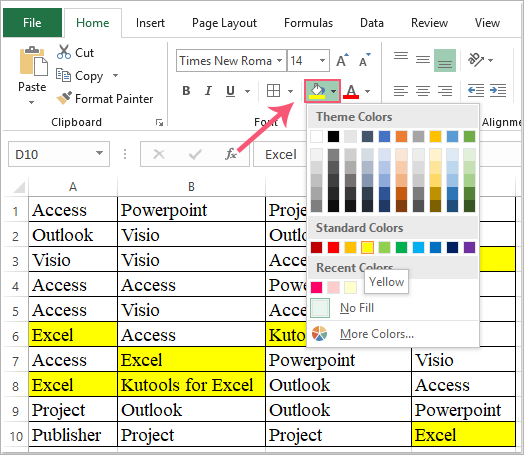
1. Selecteer het gegevensbereik dat je wilt gebruiken, en klik vervolgens op Start > Zoeken en selecteren > Zoeken, zie schermafbeelding:

2. In het dialoogvenster Zoeken en vervangen, onder het tabblad Zoeken, voer de waarde die je wilt zoeken in het vak Zoeken naar tekstvak, zie schermafbeelding:

3. Klik vervolgens op de knop Alles zoeken, in het zoekresultaatvak, klik op een item, en druk vervolgens op Ctrl + A om alle gevonden items te selecteren, zie schermafbeelding:

4. Tot slot, klik op de knop Sluiten om dit dialoogvenster te sluiten. Nu kun je een achtergrond- of lettertypekleur invullen voor deze geselecteerde waarden, zie schermafbeelding:
| Pas de achtergrondkleur toe voor de geselecteerde cellen: | Pas de lettertypekleur toe voor de geselecteerde cellen: |
 |  |
Methode 3: Achtergrond- of lettertypekleur statisch wijzigen op basis van celwaarde met Kutools voor Excel
De Super Zoeken-functie van Kutools voor Excel ondersteunt veel voorwaarden voor het zoeken van waarden, tekstreeksen, datums, formules, opgemaakte cellen enzovoort. Na het vinden en selecteren van de overeenkomende cellen, kun je de achtergrond- of lettertypekleur naar wens wijzigen.
1. Selecteer het gegevensbereik dat je wilt zoeken, en klik vervolgens op Kutools > Super Zoeken, zie schermafbeelding:

2. In het paneel Super Zoeken, voer de volgende handelingen uit:
- (1.) Klik eerst op het pictogram Waarden-optie;
- (2.) Kies het zoekbereik uit de keuzelijst Binnen, in dit geval kies ik Selectie;
- (3.) Selecteer uit de keuzelijst Type de criteria die je wilt gebruiken;
- (4.) Klik vervolgens op de knop Zoeken om alle bijbehorende resultaten in de lijstbox weer te geven;
- (5.) Klik tot slot op de knop Selecteren om de cellen te selecteren.

3. Alle cellen die voldoen aan de criteria zijn nu tegelijk geselecteerd, zie schermafbeelding:

4. En nu kun je de achtergrondkleur of lettertypekleur voor de geselecteerde cellen naar behoefte wijzigen.
Tips: Met de functie Super Zoeken kun je ook de volgende bewerkingen snel en gemakkelijk uitvoeren:
Beste productiviteitstools voor Office
Verbeter je Excel-vaardigheden met Kutools voor Excel en ervaar ongeëvenaarde efficiëntie. Kutools voor Excel biedt meer dan300 geavanceerde functies om je productiviteit te verhogen en tijd te besparen. Klik hier om de functie te kiezen die je het meest nodig hebt...
Office Tab brengt een tabbladinterface naar Office en maakt je werk veel eenvoudiger
- Activeer tabbladbewerking en -lezen in Word, Excel, PowerPoint, Publisher, Access, Visio en Project.
- Open en maak meerdere documenten in nieuwe tabbladen van hetzelfde venster, in plaats van in nieuwe vensters.
- Verhoog je productiviteit met50% en bespaar dagelijks honderden muisklikken!
Alle Kutools-invoegtoepassingen. Eén installatieprogramma
Kutools for Office-suite bundelt invoegtoepassingen voor Excel, Word, Outlook & PowerPoint plus Office Tab Pro, ideaal voor teams die werken met Office-toepassingen.
- Alles-in-één suite — invoegtoepassingen voor Excel, Word, Outlook & PowerPoint + Office Tab Pro
- Eén installatieprogramma, één licentie — in enkele minuten geïnstalleerd (MSI-ready)
- Werkt beter samen — gestroomlijnde productiviteit over meerdere Office-toepassingen
- 30 dagen volledige proef — geen registratie, geen creditcard nodig
- Beste prijs — bespaar ten opzichte van losse aanschaf van invoegtoepassingen