Meerdere overeenkomende waarden retourneren op basis van meerdere criteria in Excel (Volledige handleiding)
Excel-gebruikers komen vaak scenario's tegen waarin het nodig is om meerdere waarden te extraheren die tegelijkertijd aan verschillende criteria voldoen, en alle overeenkomende resultaten in een kolom, rij of samengevoegd in één cel weer te geven. Deze handleiding onderzoekt methoden voor alle Excel-versies, evenals de nieuwere FILTER-functie beschikbaar in Excel 365 en 2021.
Meerdere overeenkomende waarden retourneren op basis van meerdere criteria in één cel
In Excel is het extraheren van meerdere overeenkomende waarden op basis van meerdere criteria binnen één cel een veelvoorkomende uitdaging. Hier verkennen we twee efficiënte methoden.
Methode 1: Met behulp van de functie Textjoin (Excel365 / 2021,2019)
Om alle overeenkomende waarden in één cel met scheidingstekens te krijgen, kan de functie TEXTJOIN u helpen.
Voer of kopieer de volgende formule in een lege cel in, druk vervolgens op Enter (Excel 2021 en Excel 365) of Ctrl + Shift + Enter toetsen in Excel 2019 om het resultaat te krijgen:
=TEXTJOIN(", ", TRUE, IF(($A$2:$A$18=E2)*($B$2:$B$18=F2), $C$2:$C$18, ""))
- ($A$2:$A$21=E2)*($B$2:$B$21=F2) controleert of elke rij aan beide voorwaarden voldoet: 'Verkoper gelijk aan E2' en 'Maand gelijk aan F2'. Als beide voorwaarden zijn voldaan, is het resultaat 1; anders is het 0. Het sterretje * betekent dat beide voorwaarden waar moeten zijn.
- ALS(..., $C$2:$C$21, "") retourneert de productnaam als de rij overeenkomt; anders retourneert het een lege cel.
- TEKST.SAMENVOEGEN(", ", WAAR, ...) voegt alle niet-lege productnamen samen in één cel, gescheiden door ", ".
Methode 2: Met behulp van Kutools voor Excel
Kutools voor Excel biedt een krachtige maar eenvoudige oplossing waarmee je snel meerdere overeenkomsten kunt ophalen en combineren in één cel op basis van meerdere criteria zonder complexe formules.
Na installatie van Kutools voor Excel, doe het volgende:
- Selecteer het gegevensbereik waaruit je alle bijbehorende waarden wilt ophalen op basis van criteria.
- Klik vervolgens op Kutools > Samenvoegen en splitsen > Geavanceerd samenvoegen van rijen, zie screenshot:

- Configureer in het dialoogvenster Geavanceerd samenvoegen van rijen de volgende opties:
- Kies de kolomkoppen die uw overeenkomstcriteria bevatten (bijv., Verkoper en Maand). Voor elke geselecteerde kolom klikt u op Primair sleutel om ze te definiëren als uw zoekvoorwaarden.
- Klik op de kolomkop waar u de gecombineerde resultaten wilt hebben (bijv., Product). Selecteer in de sectie Combineren uw gewenste scheidingsteken (bijv., komma, spatie of aangepast scheidingsteken).
- Klik tot slot op de knop OK.


Resultaat: Kutools zal onmiddellijk alle overeenkomende waarden samenvoegen in één cel per unieke combinatie van criteria.

Meerdere overeenkomende waarden retourneren op basis van meerdere criteria in een kolom
Wanneer u meerdere overeenkomende records moet extraheren en weergeven uit een dataset op basis van verschillende voorwaarden, waarbij de resultaten in een verticale kolomindeling worden geretourneerd, biedt Excel verschillende krachtige oplossingen.
Methode 1: Met een matrixformule (voor alle versies)
U kunt de volgende matrixformule gebruiken om resultaten verticaal in een kolom te retourneren:
1. Kopieer of voer de volgende formule in een lege cel in:
=IFERROR(INDEX($C$2:$C$18, SMALL(IF(($A$2:$A$18=$E$2)*($B$2:$B$18=$F$2), ROW($C$2:$C$18)-ROW($C$2)+1), ROW(1:1))), "")2. Druk op Ctrl + Shift + Enter om het eerste overeenkomende resultaat te krijgen, selecteer dan de eerste formulecel en sleep de vulgreep naar beneden tot een lege cel wordt weergegeven. Nu zijn alle overeenkomende waarden geretourneerd zoals in de onderstaande schermopname te zien is:

- $A$2:$A$18=$E$2: Controleert of de Verkoper overeenkomt met de waarde in cel E2.
- $B$2:$B$18=$F$2: Controleert of de Maand overeenkomt met de waarde in cel F2.
- * is een logische EN-operator (beide voorwaarden moeten waar zijn).
- RIJ($C$2:$C$18)-RIJ($C$2)+1: Genereert een relatief rijnummer voor elk product.
- KLEINSTE(..., RIJ(1:1)): Haalt de n-de kleinste overeenkomende rij op (naarmate de formule naar beneden wordt getrokken).
- INDEX(...): Retourneert het product uit de overeenkomende rij.
- ALS.FOUT(..., ""): Retourneert een lege cel als er geen overeenkomsten meer zijn.
Methode 2: Met de functie Filter (Excel365 / 2021)
Als u Excel 365 of Excel 2021 gebruikt, is de FILTER-functie een uitstekende keuze om meerdere resultaten te retourneren op basis van meerdere criteria, dankzij de eenvoud, duidelijkheid en mogelijkheid om resultaten dynamisch te laten uitstromen zonder complexe matrixformules.
Kopieer of voer de onderstaande formule in een lege cel in, druk vervolgens op Enter, alle overeenkomende records worden geretourneerd op basis van de meerdere criteria.
=FILTER(C2:C18, (A2:A18=E2)*(B2:B18=F2), "No match")
- FILTER(...) retourneert alle waarden uit C2:C18 waar beide voorwaarden zijn voldaan.
- (A2:A18=E2)*(B2:B18=F2): Logische array die controleert op overeenkomende verkoper en maand.
- "Geen overeenkomst": Optioneel bericht als geen waarden worden gevonden.
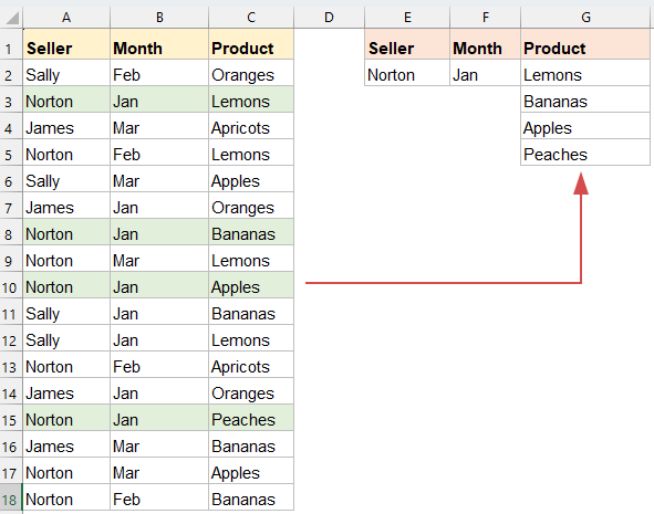
Meerdere overeenkomende waarden retourneren op basis van meerdere criteria in een rij
Excel-gebruikers moeten vaak meerdere waarden extraheren uit een dataset die aan verschillende voorwaarden voldoen en deze horizontaal weergeven (in een rij). Dit is nuttig voor het maken van dynamische rapporten, dashboards of samenvattingstabellen waar de verticale ruimte beperkt is. In deze sectie verkennen we twee krachtige methoden.
Methode 1: Met een matrixformule (voor alle versies)
Traditionele matrixformules stellen u in staat meerdere overeenkomende waarden te extraheren met behulp van INDEX, KLEINSTE, ALS en KOLOM-functies. In tegenstelling tot verticale extractie (kolombased), passen we de formule aan om resultaten in een rij te retourneren.
1. Kopieer of voer de onderstaande formule in een lege cel in:
=IFERROR(INDEX($C$2:$C$18, SMALL(IF(($A$2:$A$18=$E$2)*($B$2:$B$18=$F$2), ROW($C$2:$C$18)-ROW($C$2)+1), COLUMN(A1))), "")2. Druk op Ctrl + Shift + Enter om het eerste overeenkomende resultaat te krijgen, selecteer dan de eerste formulecel en sleep de formule naar rechts over kolommen om alle resultaten op te halen.

- $A$2:$A$18=$E$2: Controleert of de Verkoper overeenkomt.
- $B$2:$B$18=$F$2: Controleert of de Maand overeenkomt.
- *: Logische EN—beide voorwaarden moeten waar zijn.
- RIJ($C$2:$C$18)-RIJ($C$2)+1: Creëert relatieve rijnummers.
- KOLOM(A1): Past aan welke overeenkomst moet worden geretourneerd, afhankelijk van hoe ver de formule naar rechts is gesleept.
- ALS.FOUT(...): Voorkomt fouten zodra overeenkomsten zijn uitgeput.
Methode 2: Met de functie Filter (Excel365 / 2021)
Kopieer of voer de onderstaande formule in een lege cel in, druk vervolgens op Enter, alle overeenkomende waarden worden geëxtraheerd en in een rij geplaatst. Zie schermopname:
=TRANSPOSE(FILTER(C2:C18, (A2:A18=E2)*(B2:B18=F2), "No match"))
- FILTER(...): Haalt overeenkomende waarden op uit kolom C op basis van de twee voorwaarden.
- (A2:A18=E2)*(B2:B18=F2): Beide voorwaarden moeten waar zijn.
- TRANSPOSE(...): Converteert de verticale array geretourneerd door FILTER in een horizontale array.
🔚 Conclusie
Het ophalen van meerdere overeenkomende waarden op basis van meerdere criteria in Excel kan op verschillende manieren worden bereikt, afhankelijk van hoe u de resultaten wilt weergeven—ofwel in een kolom, een rij of binnen één cel.
- Voor gebruikers met Excel 365 of Excel 2021 biedt de FILTER-functie een moderne, dynamische en elegante oplossing die complexiteit minimaliseert.
- Voor gebruikers van oudere versies blijven matrixformules krachtige tools, hoewel ze wat meer instelling en zorg vereisen.
- Daarnaast, als u resultaten wilt consolideren in één cel of een no-code-oplossing prefereert, kunnen de functie TEKST.SAMENVOEGEN of derden tools zoals Kutools voor Excel het proces aanzienlijk vereenvoudigen.
Kies de methode die het beste past bij uw versie van Excel en uw gewenste indeling, en u bent goed uitgerust om multi-criteria lookups efficiënt en nauwkeurig af te handelen. Als u geïnteresseerd bent in het verkennen van meer Excel-tips en -trucs, onze website biedt duizenden tutorials om u te helpen Excel te beheersen.
Meer gerelateerde artikelen:
- Retourneer Meerdere Zoekwaarden In Eén Cel Gescheiden Door Komma’s
- In Excel kunnen we de functie VLOOKUP toepassen om de eerste overeenkomende waarde uit tabelcellen te retourneren, maar soms moeten we alle overeenkomende waarden extraheren en vervolgens gescheiden door een specifiek scheidingsteken, zoals komma, streepje, etc… in één cel plaatsen zoals in de volgende schermopname te zien is. Hoe kunnen we meerdere zoekwaarden krijgen en retourneren in één cel gescheiden door komma’s in Excel?
- Zoekopdracht Uitvoeren En Meerdere Overeenkomende Waarden Tegelijk Retourneren In Google Sheet
- De normale VLOOKUP-functie in Google Sheets kan u helpen om de eerste overeenkomende waarde te vinden en retourneren op basis van een gegeven dataset. Maar soms moet u mogelijk VLOOKUP uitvoeren en alle overeenkomende waarden retourneren zoals in de volgende schermopname te zien is. Heeft u goede en eenvoudige manieren om deze taak in Google Sheets op te lossen?
- Zoekopdracht Uitvoeren En Meerdere Waarden Van Keuzelijst Retourneren
- In Excel, hoe kunt u VLOOKUP uitvoeren en meerdere bijbehorende waarden retourneren van een keuzelijst, wat betekent dat wanneer u een item uit de keuzelijst selecteert, alle bijbehorende waarden tegelijk worden weergegeven zoals in de volgende schermopname te zien is. In dit artikel zal ik stap voor stap de oplossing introduceren.
- Zoekopdracht Uitvoeren En Meerdere Waarden Verticaal Retourneren In Excel
- Normaal gesproken kunt u de functie VLOOKUP gebruiken om de eerste bijbehorende waarde te krijgen, maar soms wilt u alle passende records retourneren op basis van een specifiek criterium. In dit artikel zal ik bespreken hoe u VLOOKUP kunt gebruiken en alle overeenkomende waarden verticaal, horizontaal of in één enkele cel kunt retourneren.
- Zoekopdracht Uitvoeren En Overeenkomende Gegevens Tussen Twee Waarden Retourneren In Excel
- In Excel kunnen we de normale VLOOKUP-functie toepassen om de bijbehorende waarde te krijgen op basis van een gegeven dataset. Maar soms willen we VLOOKUP uitvoeren en de overeenkomende waarde tussen twee waarden retourneren zoals in de volgende schermopname te zien is, hoe zou u deze taak in Excel kunnen aanpakken?
Beste productiviteitstools voor Office
Verbeter je Excel-vaardigheden met Kutools voor Excel en ervaar ongeëvenaarde efficiëntie. Kutools voor Excel biedt meer dan300 geavanceerde functies om je productiviteit te verhogen en tijd te besparen. Klik hier om de functie te kiezen die je het meest nodig hebt...
Office Tab brengt een tabbladinterface naar Office en maakt je werk veel eenvoudiger
- Activeer tabbladbewerking en -lezen in Word, Excel, PowerPoint, Publisher, Access, Visio en Project.
- Open en maak meerdere documenten in nieuwe tabbladen van hetzelfde venster, in plaats van in nieuwe vensters.
- Verhoog je productiviteit met50% en bespaar dagelijks honderden muisklikken!
Alle Kutools-invoegtoepassingen. Eén installatieprogramma
Kutools for Office-suite bundelt invoegtoepassingen voor Excel, Word, Outlook & PowerPoint plus Office Tab Pro, ideaal voor teams die werken met Office-toepassingen.
- Alles-in-één suite — invoegtoepassingen voor Excel, Word, Outlook & PowerPoint + Office Tab Pro
- Eén installatieprogramma, één licentie — in enkele minuten geïnstalleerd (MSI-ready)
- Werkt beter samen — gestroomlijnde productiviteit over meerdere Office-toepassingen
- 30 dagen volledige proef — geen registratie, geen creditcard nodig
- Beste prijs — bespaar ten opzichte van losse aanschaf van invoegtoepassingen