Hoe kun je met VLOOKUP een waarde opzoeken en tegelijkertijd de achtergrondkleur retourneren in Excel?
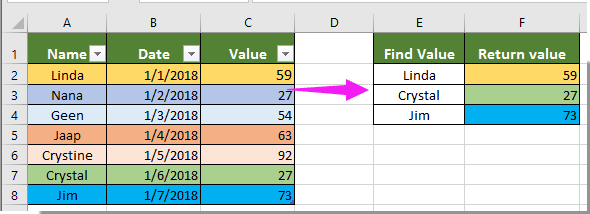
Stel dat je een tabel hebt zoals in onderstaande schermafbeelding. Nu wil je controleren of een bepaalde waarde voorkomt in kolom A en vervolgens de bijbehorende waarde retourneren samen met de achtergrondkleur in kolom C. Hoe kun je dit bereiken? De methode in dit artikel kan je helpen het probleem op te lossen.
VLOOKUP en retourneer achtergrondkleur met zoekwaarde via een door de gebruiker gedefinieerde functie
Volg de volgende stappen om een waarde op te zoeken en de bijbehorende waarde samen met de achtergrondkleur in Excel te retourneren.
1. Open het werkblad dat de waarde bevat die je wilt opzoeken, klik met de rechtermuisknop op het tabblad van het blad en selecteer Weergave Code in het contextmenu. Zie screenshot:

2. Kopieer in het venster Microsoft Visual Basic for Applications dat wordt geopend de onderstaande VBA-code naar het Code-venster.
VBA-code 1: VLOOKUP en retourneer achtergrondkleur met de zoekwaarde
Sub Worksheet_Change(ByVal Target As Range)
    Dim I As Long
    Dim xKeys As Long
    Dim xDicStr As String
    On Error Resume Next
    Application.ScreenUpdating = False
    xKeys = UBound(xDic.Keys)
    If xKeys >= 0 Then
        For I = 0 To UBound(xDic.Keys)
            xDicStr = xDic.Items(I)
            If xDicStr <> "" Then
                Range(xDic.Keys(I)).Interior.Color = _
                Range(xDic.Items(I)).Interior.Color
            Else
                Range(xDic.Keys(I)).Interior.Color = xlNone
            End If
        Next
        Set xDic = Nothing
    End If
    Application.ScreenUpdating = True
End Sub
3. Klik vervolgens op Invoegen > Module en kopieer de onderstaande VBA-code 2 naar het Module-venster.
VBA-code 2: VLOOKUP en retourneer achtergrondkleur met de zoekwaarde
Public xDic As New Dictionary
Function LookupKeepColor (ByRef FndValue, ByRef LookupRng As Range, ByRef xCol As Long)
    Dim xFindCell As Range
    On Error Resume Next
    Set xFindCell = LookupRng.Find(FndValue, , xlValues, xlWhole)
    If xFindCell Is Nothing Then
        LookupKeepColor = ""
        xDic.Add Application.Caller.Address, ""
    Else
        LookupKeepColor = xFindCell.Offset(0, xCol - 1).Value
        xDic.Add Application.Caller.Address, xFindCell.Offset(0, xCol - 1).Address
    End If
End Function
4. Nadat je de twee codes hebt ingevoegd, klik je op Tools > Referenties. Vink vervolgens het vakje Microsoft Script Runtime aan in het dialoogvenster Referenties – VBAProject. Zie screenshot:

5. Druk op Alt + Q om het venster Microsoft Visual Basic for Applications te sluiten en terug te keren naar het werkblad.
6. Selecteer een lege cel naast de zoekwaarde en voer vervolgens de formule =LookupKeepColor(E2,$A$1:$C$8,3) in de Formulebalk in en druk op Enter.

Opmerking: In de formule bevat E2 de waarde die je wilt opzoeken, $A$1:$C$8 is het tabelbereik en het getal 3 betekent dat de bijbehorende waarde die je wilt retourneren zich in de derde kolom van de tabel bevindt. Pas deze waarden indien nodig aan.
7. Blijf de eerste resultaatcel selecteren en sleep de vulgreep naar beneden om alle resultaten samen met hun achtergrondkleur te krijgen. Zie screenshot.

Gerelateerde artikelen:
- Hoe kopieer je de bronopmaak van de zoekcel wanneer je VLOOKUP gebruikt in Excel?
- Hoe retourneer je datumformaat in plaats van een getal bij het gebruik van VLOOKUP in Excel?
- Hoe gebruik je VLOOKUP en som in Excel?
- Hoe retourneer je een waarde in een aangrenzende of volgende cel met VLOOKUP in Excel?
- Hoe gebruik je VLOOKUP om waar of onwaar / ja of nee te retourneren in Excel?
Beste productiviteitstools voor Office
Verbeter je Excel-vaardigheden met Kutools voor Excel en ervaar ongeëvenaarde efficiëntie. Kutools voor Excel biedt meer dan300 geavanceerde functies om je productiviteit te verhogen en tijd te besparen. Klik hier om de functie te kiezen die je het meest nodig hebt...
Office Tab brengt een tabbladinterface naar Office en maakt je werk veel eenvoudiger
- Activeer tabbladbewerking en -lezen in Word, Excel, PowerPoint, Publisher, Access, Visio en Project.
- Open en maak meerdere documenten in nieuwe tabbladen van hetzelfde venster, in plaats van in nieuwe vensters.
- Verhoog je productiviteit met50% en bespaar dagelijks honderden muisklikken!
Alle Kutools-invoegtoepassingen. Eén installatieprogramma
Kutools for Office-suite bundelt invoegtoepassingen voor Excel, Word, Outlook & PowerPoint plus Office Tab Pro, ideaal voor teams die werken met Office-toepassingen.
- Alles-in-één suite — invoegtoepassingen voor Excel, Word, Outlook & PowerPoint + Office Tab Pro
- Eén installatieprogramma, één licentie — in enkele minuten geïnstalleerd (MSI-ready)
- Werkt beter samen — gestroomlijnde productiviteit over meerdere Office-toepassingen
- 30 dagen volledige proef — geen registratie, geen creditcard nodig
- Beste prijs — bespaar ten opzichte van losse aanschaf van invoegtoepassingen