Hoe conditionele opmaak te gebruiken op basis van een ander werkblad in Google Sheets?
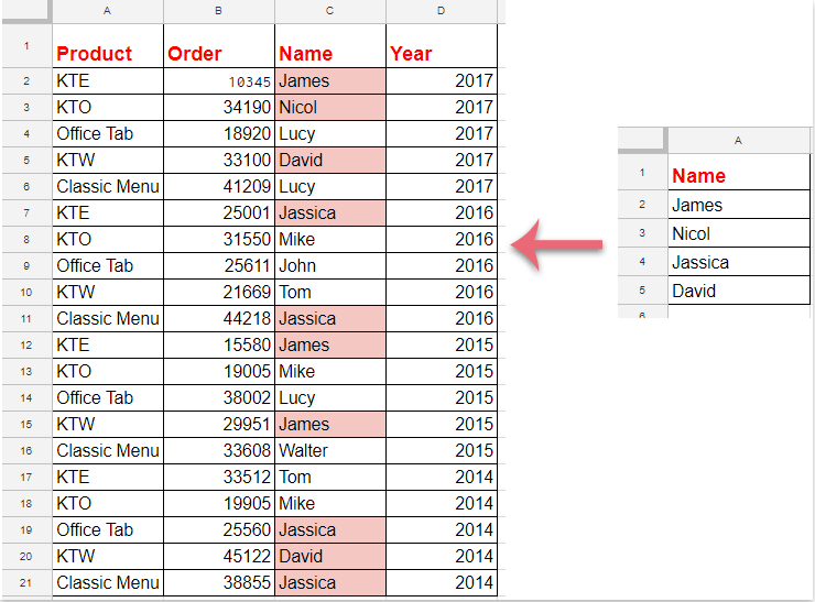
Conditionele opmaak is een handige functie in Google Sheets waarmee je cellen automatisch kunt markeren op basis van specifieke criteria, waardoor het gemakkelijker wordt om je gegevens te analyseren en te visualiseren. Soms wil je cellen niet markeren op basis van waarden binnen hetzelfde werkblad, maar wil je je opmaakregels baseren op een referentielijst of criteria die zijn opgeslagen in een ander werkblad. Bijvoorbeeld, je wilt misschien cellen in één werkblad markeren die ook voorkomen in een lijst die wordt onderhouden in een ander werkblad, zoals geïllustreerd in de onderstaande schermafbeelding. Dit soort taak komt vaak voor wanneer je werkt met gekoppelde gegevens, zoals het vergelijken van huidige verkoopcijfers met een hoofdproductlijst, of het controleren op dubbele invoer tegenover een andere gegevensbron. Het instellen van dergelijke conditionele opmaak in Google Sheets—vooral bij het raadplegen van gegevens uit verschillende werkbladen—kan verwarrend zijn als je het nog nooit eerder hebt gedaan. De onderstaande handleiding zal je, stap voor stap, een eenvoudige aanpak laten zien om dit te bereiken.
Conditionele opmaak om cellen te markeren op basis van een lijst uit een ander werkblad in Google Sheets
Deze methode laat je een regel voor conditionele opmaak instellen om cellen in je actieve werkblad te markeren als ze voorkomen in een gespecificeerde lijst uit een ander werkblad. Dergelijke cross-sheet conditionele opmaak is vooral handig voor dynamisch datamonitoring en het behouden van consistentie tussen gerelateerde datasets.
Volg deze gedetailleerde stappen om dit proces te voltooien:
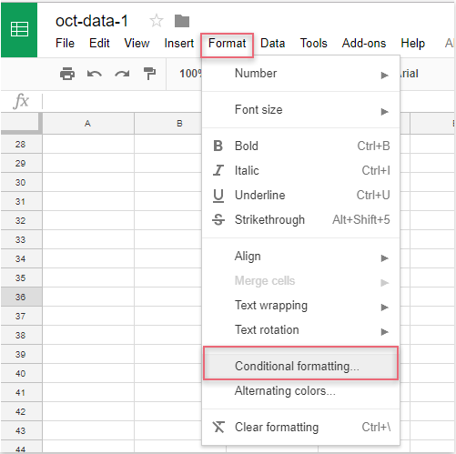
1. Open je doelwerkblad, klik vervolgens op het menu Opmaak bovenaan, en selecteer Conditionele opmaak. Het paneel Conditionele opmaakregels zal openen aan de rechterkant van je scherm.
2. Neem de volgende acties op het paneel Conditionele opmaakregels:
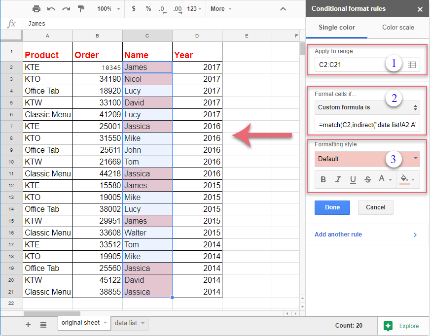
(1.) Klik op de ![]() knop naast het veld "Toepassen op bereik". Selecteer het bereik van cellen dat je wilt markeren. Als je bijvoorbeeld alle waarden in kolom C vanaf rij 2 wilt formatteren, selecteer dan C2:C. Het selecteren van een geschikt bereik zorgt ervoor dat alleen de bedoelde cellen worden geëvalueerd voor opmaak.
knop naast het veld "Toepassen op bereik". Selecteer het bereik van cellen dat je wilt markeren. Als je bijvoorbeeld alle waarden in kolom C vanaf rij 2 wilt formatteren, selecteer dan C2:C. Het selecteren van een geschikt bereik zorgt ervoor dat alleen de bedoelde cellen worden geëvalueerd voor opmaak.
(2.) Kies in het vervolgmenu 'Celopmaak instellen als' de optie Aangepaste formule is. Voer de volgende formule in het daarvoor bestemde vak in: =match(C2,indirect("data list!A2:A"),0). Deze formule controleert of elke cel in kolom C overeenkomt met een waarde in het bereik A2:A van het werkblad "data list".
(3.) Selecteer onder Opmaakstijl je gewenste opmaak, zoals het vullen van de cel met een specifieke kleur of het wijzigen van het lettertype. Je kunt de stijl onmiddellijk in je werkblad bekijken voordat je deze toepast.
Opmerking: In de bovenstaande formule verwijst C2 naar de eerste cel in je geselecteerde bereik (pas aan als je gegevens beginnen in een andere rij of kolom), en data list!A2:A verwijst naar de naam van het werkblad (“data list”) en het bijbehorende bereik (A2:A) waar je lijst uit een ander werkblad is opgeslagen. Zorg ervoor dat de celverwijzing in de formule overeenkomt met de linkerbovenste cel van je geselecteerde bereik, anders wordt de opmaak mogelijk niet correct toegepast. Als je gegevenslijstbereik anders is, vergeet dan niet om het in de formule bij te werken (bijvoorbeeld, “data list!B2:B”).
3. Zodra je de regel hebt ingesteld, worden overeenkomende cellen in je gekozen bereik direct gemarkeerd op basis van de lijst uit het andere werkblad. Bekijk de preview, klik vervolgens op Gereed onderaan het paneel Conditionele opmaakregels om je opmaak toe te passen en op te slaan.
Tips en probleemoplossing:
- Controleer tweemaal op typfouten in je formule, vooral in werkbladnamen en bereikverwijzingen—onjuiste verwijzingen zijn een veelvoorkomende reden waarom regels niet worden toegepast.
- Als je gegevenslijst lege cellen bevat, zal de functie
MATCHeen#N/Bfout retourneren voor niet-overeenkomende waarden, maar dit is verwacht gedrag en heeft geen invloed op het markeren van overeenkomende items. - Wanneer je opmaak kopieert naar een nieuw werkblad of bereiken aanpast, zorg er dan voor dat je ook de celverwijzingen in je aangepaste formule dienovereenkomstig bijwerkt.
- De opmaak wordt automatisch bijgewerkt als je later items toevoegt of verwijdert uit je referentielijst.
- Het werkblad en het bereik dat in je formule wordt verwezen bestaan en correct zijn gespeld.
- De eerste cel in je formule overeenkomt met de eerste cel van je geselecteerde bereik.
- Alle benodigde toestemmingen voor cross-sheet toegang binnen je spreadsheet beschikbaar zijn—deze methode werkt binnen een enkel multi-werkblad Google Sheets bestand, niet tussen verschillende bestanden.
Als alternatief, als je gegevensstructuur of vereisten complexer zijn—bijvoorbeeld als je meerdere kolommen moet vergelijken, gedeeltelijke overeenkomsten moet toestaan, of geavanceerdere zoekacties moet uitvoeren—kan het gebruik van hulpkolommen met COUNTIF- of VLOOKUP-formules, of het gebruik van Google Apps Script (aangepaste JavaScript-code), ook flexibele oplossingen bieden voor conditionele opmaak.
Samenvattend, het instellen van conditionele opmaak op basis van een ander werkblad is uiterst effectief voor het controleren van lijsten, het bijhouden van duplicaten en diverse cross-sheet gegevensvalidaties—alles binnen Google Sheets. Controleer altijd je formule-invoer, verwijzingsbereiken en opmaakregels voor soepele en nauwkeurige resultaten.

Ontdek de Magie van Excel met Kutools AI
- Slimme Uitvoering: Voer celbewerkingen uit, analyseer gegevens en maak diagrammen – allemaal aangestuurd door eenvoudige commando's.
- Aangepaste Formules: Genereer op maat gemaakte formules om uw workflows te versnellen.
- VBA-codering: Schrijf en implementeer VBA-code moeiteloos.
- Formule-uitleg: Begrijp complexe formules gemakkelijk.
- Tekstvertaling: Overbrug taalbarrières binnen uw spreadsheets.
Beste productiviteitstools voor Office
Verbeter je Excel-vaardigheden met Kutools voor Excel en ervaar ongeëvenaarde efficiëntie. Kutools voor Excel biedt meer dan300 geavanceerde functies om je productiviteit te verhogen en tijd te besparen. Klik hier om de functie te kiezen die je het meest nodig hebt...
Office Tab brengt een tabbladinterface naar Office en maakt je werk veel eenvoudiger
- Activeer tabbladbewerking en -lezen in Word, Excel, PowerPoint, Publisher, Access, Visio en Project.
- Open en maak meerdere documenten in nieuwe tabbladen van hetzelfde venster, in plaats van in nieuwe vensters.
- Verhoog je productiviteit met50% en bespaar dagelijks honderden muisklikken!
Alle Kutools-invoegtoepassingen. Eén installatieprogramma
Kutools for Office-suite bundelt invoegtoepassingen voor Excel, Word, Outlook & PowerPoint plus Office Tab Pro, ideaal voor teams die werken met Office-toepassingen.
- Alles-in-één suite — invoegtoepassingen voor Excel, Word, Outlook & PowerPoint + Office Tab Pro
- Eén installatieprogramma, één licentie — in enkele minuten geïnstalleerd (MSI-ready)
- Werkt beter samen — gestroomlijnde productiviteit over meerdere Office-toepassingen
- 30 dagen volledige proef — geen registratie, geen creditcard nodig
- Beste prijs — bespaar ten opzichte van losse aanschaf van invoegtoepassingen