Hoe maak je een afhankelijke keuzelijst in Google Sheets?
Het invoegen van een normale keuzelijst in Google Sheets is misschien eenvoudig voor je, maar soms moet je mogelijk een afhankelijke keuzelijst maken, waarbij de tweede lijst afhangt van de selectie in de eerste lijst. Hoe kun je deze taak in Google Sheets aanpakken?
Maak een afhankelijke keuzelijst in Google Sheets
Maak een afhankelijke keuzelijst in Google Sheets
Volg deze stappen om een afhankelijke keuzelijst te maken in Google Sheets:
1. Voeg eerst de basis keuzelijst in, selecteer een cel waar je de eerste keuzelijst wilt plaatsen en klik vervolgens op Gegevens > Gegevensvalidatie, zie screenshot:

2. In het pop-upvenster Gegevensvalidatie dialoogvenster, selecteer Lijst uit een bereik uit de keuzelijst naast de Criteria sectie, en klik vervolgens op ![]() knop om de celwaarden te selecteren waarop je de eerste keuzelijst wilt baseren, zie screenshot:
knop om de celwaarden te selecteren waarop je de eerste keuzelijst wilt baseren, zie screenshot:

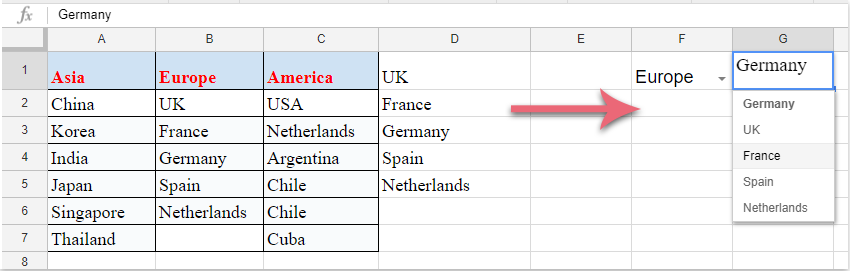
3. Klik vervolgens op de knop Opslaan, de eerste keuzelijst is gemaakt. Kies een item uit de aangemaakte keuzelijst en voer vervolgens deze formule in: =arrayformula(if(F1=A1,A2:A7,if(F1=B1,B2:B6,if(F1=C1,C2:C7,"")))) in een lege cel naast de gegevenskolommen, druk vervolgens op Enter-toets, alle overeenkomende waarden op basis van het eerste keuzelijstitem worden meteen weergegeven, zie screenshot:
Opmerking: In de bovenstaande formule: F1 is de cel van de eerste keuzelijst, A1, B1 en C1 zijn de items van de eerste keuzelijst, A2:A7, B2:B6 en C2:C7 zijn de celwaarden waarop de tweede keuzelijst is gebaseerd. Je kunt ze naar eigen wens wijzigen.

4. Vervolgens kun je de tweede afhankelijke keuzelijst maken, klik op een cel waar je de tweede keuzelijst wilt plaatsen, en klik vervolgens op Gegevens > Gegevensvalidatie om naar het dialoogvenster Gegevensvalidatie te gaan, kies Lijst uit een bereik uit de keuzelijst naast de sectie Criteria, en ga door met het klikken op de knop om de formulecellen te selecteren die de overeenkomende resultaten van het eerste keuzelijstitem zijn, zie screenshot:

5. Klik tot slot op de knop Opslaan, en de tweede afhankelijke keuzelijst is succesvol aangemaakt zoals in de volgende schermafbeelding wordt getoond:
Beste productiviteitstools voor Office
Verbeter je Excel-vaardigheden met Kutools voor Excel en ervaar ongeëvenaarde efficiëntie. Kutools voor Excel biedt meer dan300 geavanceerde functies om je productiviteit te verhogen en tijd te besparen. Klik hier om de functie te kiezen die je het meest nodig hebt...
Office Tab brengt een tabbladinterface naar Office en maakt je werk veel eenvoudiger
- Activeer tabbladbewerking en -lezen in Word, Excel, PowerPoint, Publisher, Access, Visio en Project.
- Open en maak meerdere documenten in nieuwe tabbladen van hetzelfde venster, in plaats van in nieuwe vensters.
- Verhoog je productiviteit met50% en bespaar dagelijks honderden muisklikken!
Alle Kutools-invoegtoepassingen. Eén installatieprogramma
Kutools for Office-suite bundelt invoegtoepassingen voor Excel, Word, Outlook & PowerPoint plus Office Tab Pro, ideaal voor teams die werken met Office-toepassingen.
- Alles-in-één suite — invoegtoepassingen voor Excel, Word, Outlook & PowerPoint + Office Tab Pro
- Eén installatieprogramma, één licentie — in enkele minuten geïnstalleerd (MSI-ready)
- Werkt beter samen — gestroomlijnde productiviteit over meerdere Office-toepassingen
- 30 dagen volledige proef — geen registratie, geen creditcard nodig
- Beste prijs — bespaar ten opzichte van losse aanschaf van invoegtoepassingen