Maak een zoekvak in Excel – Een stap-voor-stapgids

Het maken van een zoekvak in Excel verbetert de functionaliteit van uw spreadsheets door het eenvoudiger te maken om specifieke gegevens snel te filteren en te benaderen. Deze handleiding behandelt verschillende methoden om een zoekvak te implementeren, afgestemd op verschillende versies van Excel. Of u nu een beginner of een gevorderde gebruiker bent, deze stappen helpen u een dynamisch zoekvak in te stellen met behulp van functies zoals de FILTER-functie, Voorwaardelijke opmaak en diverse formules.

• Maak eenvoudig een zoekvak met de FILTER-functie
  (beschikbaar in Excel 2019 en later, Excel voor Microsoft 365)
• Maak een zoekvak met Voorwaardelijke opmaak
  (beschikbaar in alle Excel-versies)
• Maak een zoekvak met formulecombinaties
  (beschikbaar in alle Excel-versies)

Maak eenvoudig een zoekvak met de FILTER-functie

• Deze functie werkt automatisch bij wanneer uw gegevens veranderen.
• De FILTER-functie kan elk aantal resultaten retourneren, van een enkele rij tot duizenden, afhankelijk van hoeveel items in uw dataset voldoen aan de ingestelde criteria.

Hier zal ik u laten zien hoe u de FILTER-functie kunt gebruiken om een zoekvak in Excel te maken.

Stap 1: Voeg een tekstvak in en configureer eigenschappen

1. Ga naar het tabblad "Developer", klik op "Insert" > "Text Box (ActiveX Control)".
   Tip: Als het tabblad "Developer" niet wordt weergegeven op de lintbalk, kunt u het inschakelen door de instructies in deze handleiding te volgen: Hoe toon/vertoon je het developer-tabblad in de Excel-lintbalk?
   
2. De cursor verandert in een kruis, waarna u de cursor moet slepen om het tekstvak te tekenen op de locatie in het werkblad waar u het tekstvak wilt plaatsen. Na het tekenen van het tekstvak laat u de muis los.
   
3. Klik met de rechtermuisknop op het tekstvak en selecteer "Properties" uit het contextmenu.
   
4. Voer in het "Properties"-paneel de celreferentie in het veld "LinkedCell" in om het tekstvak aan een cel te koppelen. Bijvoorbeeld, door "J2" in te voeren, zorgt u ervoor dat elke ingevoerde gegevens in het tekstvak automatisch worden bijgewerkt in cel J2, en vice versa.
   
5. Klik op "Design Mode" onder het tabblad "Developer" om de "Design Mode" te verlaten.
   

Het tekstvak staat nu toe om tekst in te voeren.

Stap 2: Pas de FILTER-functie toe

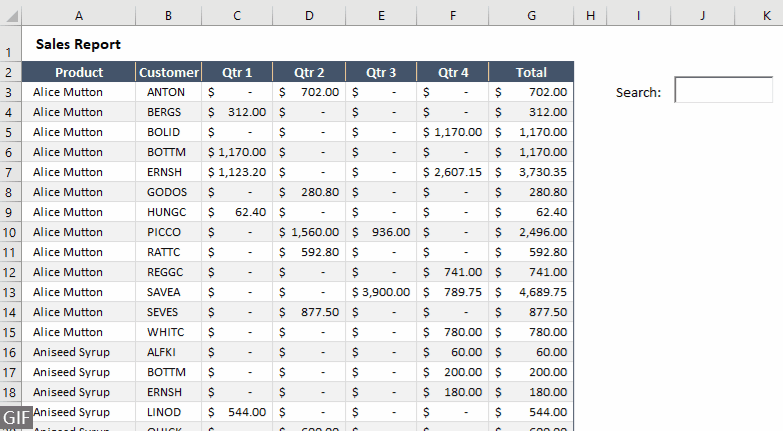
1. Kopieer voordat u de FILTER-functie gebruikt de originele koprij naar een nieuw gebied. Hier plaats ik de koprij onder het zoekvak.
   Tip: Deze aanpak stelt gebruikers in staat om de resultaten duidelijk te zien onder dezelfde kolomkoppen als de originele gegevens.
   
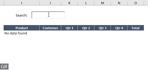
2. Selecteer de cel onder de eerste kop (bijv. I5 in dit voorbeeld), voer de volgende formule in en druk op de "Enter"-toets om het resultaat te krijgen.

   =FILTER(Sheet2!$A$5:$G$281,Sheet2!$B$5:$B$281=J2,"No data found")

   
   Zoals te zien is in de bovenstaande schermafbeelding, omdat er momenteel geen invoer is in het tekstvak, geeft de formule het resultaat "Geen gegevens gevonden" weer in I5.

Resultaat: Test het zoekvak

Laten we nu het zoekvak testen. In dit voorbeeld, wanneer ik de naam van een klant in het zoekvak invoer, worden de bijbehorende resultaten gefilterd en onmiddellijk weergegeven.

Maak een zoekvak met Voorwaardelijke opmaak

Voorwaardelijke opmaak kan worden gebruikt om gegevens die overeenkomen met een zoekterm te markeren, waardoor indirect een zoekvak-effect wordt gecreëerd. Deze methode filtert gegevens niet uit, maar leidt u visueel naar de relevante cellen. In deze sectie wordt uitgelegd hoe u een zoekvak maakt met behulp van Voorwaardelijke opmaak in Excel.

Stap 1: Voeg een tekstvak in en configureer eigenschappen

1. Ga naar het tabblad "Developer", klik op "Insert" > "Text Box (ActiveX Control)".
   Tip: Als het tabblad "Developer" niet wordt weergegeven op de lintbalk, kunt u het inschakelen door de instructies in deze handleiding te volgen: Hoe toon/vertoon je het developer-tabblad in de Excel-lintbalk?
   
2. De cursor verandert in een kruis, waarna u de cursor moet slepen om het tekstvak te tekenen op de locatie in het werkblad waar u het tekstvak wilt plaatsen. Na het tekenen van het tekstvak laat u de muis los.
   
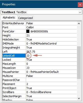
3. Klik met de rechtermuisknop op het tekstvak en selecteer "Properties" uit het contextmenu.
   
4. Voer in het "Properties"-paneel de celreferentie in het veld "LinkedCell" in om het tekstvak aan een cel te koppelen. Bijvoorbeeld, door "J3" in te voeren, zorgt u ervoor dat elke ingevoerde gegevens in het tekstvak automatisch worden bijgewerkt in cel J3, en vice versa.
   
5. Klik op "Design Mode" onder het tabblad "Developer" om de "Design Mode" te verlaten.
   

Het tekstvak staat nu toe om tekst in te voeren.

Stap 2: Pas Voorwaardelijke opmaak toe voor het zoeken van gegevens

1. Selecteer het hele gegevensbereik dat moet worden doorzocht. Hier selecteer ik het bereik A3:G279.
2. Onder het tabblad "Home", klik op "Voorwaardelijke opmaak" > "Nieuwe regel".
   
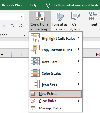
3. In het dialoogvenster "Nieuwe opmaakregel":
   1. Selecteer "Gebruik een formule om te bepalen welke cellen moeten worden opgemaakt" in de opties "Selecteer een regeltype".
   2. Voer de volgende formule in het vak "Formatteer waarden waar deze formule waar is" in.

      =$B3=$J$3

      Hier vertegenwoordigt "$B3" de eerste cel in de kolom die u wilt matchen met de zoekcriteria in het geselecteerde bereik, en "$J$3" is de cel die is gekoppeld aan het zoekvak.
   3. Klik op de knop "Opmaak" om een vulkleur voor de zoekresultaten te specificeren.
   4. Klik op de knop "OK". Zie schermafbeelding:
      

Resultaat

Laten we nu het zoekvak testen. In dit voorbeeld, wanneer ik de naam van een klant in het zoekvak invoer, worden de bijbehorende rijen die deze klant in kolom B bevatten, onmiddellijk gemarkeerd met de gespecificeerde vulkleur.

Maak een zoekvak met formulecombinaties

Als u niet de nieuwste versie van Excel gebruikt en liever niet alleen rijen wilt markeren, kan de in deze sectie beschreven methode nuttig zijn. U kunt een combinatie van Excel-formules gebruiken om een functioneel zoekvak te maken in elke versie van Excel. Volg de onderstaande stappen.

Stap 1: Maak een lijst met unieke waarden uit de zoekkolom

1. In dit geval selecteer en kopieer ik het bereik "B4:B281" naar een nieuw werkblad.
2. Na het plakken van het bereik in een nieuw werkblad, houdt u de geplakte gegevens geselecteerd, gaat u naar het tabblad "Data" en selecteert u "Dubbele items verwijderen".
   
3. Klik in het dialoogvenster "Dubbele items verwijderen" op de knop "OK".
   
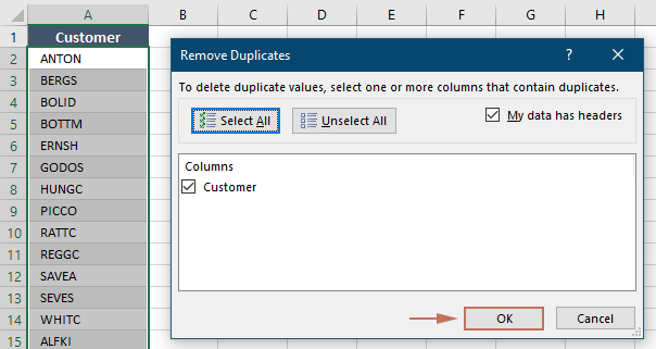
4. Er verschijnt vervolgens een "Microsoft Excel"-promptvenster dat laat zien hoeveel duplicaten zijn verwijderd. Klik op "OK".
   
5. Nadat de duplicaten zijn verwijderd, selecteert u alle unieke waarden in de lijst, met uitzondering van de kop, en wijst u een naam toe aan dit bereik door deze in het vak "Naam" in te voeren. Hier heb ik het bereik genaamd "Customer".
   

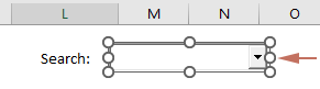
Stap 2: Voeg een keuzelijst in en configureer eigenschappen

1. Ga terug naar het werkblad met de dataset die u wilt doorzoeken. Ga naar het tabblad "Developer", klik op "Insert" > "Combo Box (ActiveX Control)".
   Tip: Als het tabblad "Developer" niet wordt weergegeven op de lintbalk, kunt u het inschakelen door de instructies in deze handleiding te volgen: Hoe toon/vertoon je het developer-tabblad in de Excel-lintbalk?
   
2. De cursor verandert in een kruis, waarna u de cursor moet slepen om de keuzelijst te tekenen op de locatie in het werkblad waar u het zoekvak wilt plaatsen. Na het tekenen van de keuzelijst laat u de muis los.
   
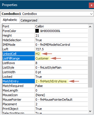
3. Klik met de rechtermuisknop op de keuzelijst en selecteer "Properties" uit het contextmenu.
   
4. In het "Properties"-paneel:
   1. Koppel de keuzelijst aan een cel door de celreferentie in het veld "LinkedCell" in te voeren. Hier typ ik "M2".
      Tip: Door dit veld te specificeren, zorgt u ervoor dat elke ingevoerde gegevens in de keuzelijst automatisch worden bijgewerkt in cel M2, en vice versa.
   2. Voer in het veld "ListFillRange" de "bereiknaam" in die u hebt gespecificeerd voor de unieke lijst in Stap 1.
   3. Wijzig het veld "MatchEntry" naar "2 – fmMatchEntryNone".
   4. Sluit het "Properties"-paneel.
      
5. Klik op "Design Mode" onder het tabblad "Developer" om de Design Mode te verlaten.
   

U kunt nu elk item in de keuzelijst selecteren of tekst invoeren om te zoeken.

Stap 3: Pas formules toe

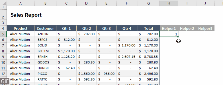
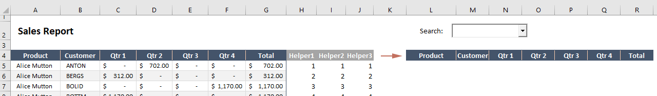
1. Maak drie hulpcolumnen naast het originele gegevensbereik. Zie schermafbeelding:
   
2. Voer in de cel (H5) onder de kop van de eerste hulpcolumnen de volgende formule in en druk op "Enter".

   =ROWS($B$5:B5)

   Hier is "B5" de cel die de naam van de eerste klant in de kolom bevat die moet worden doorzocht.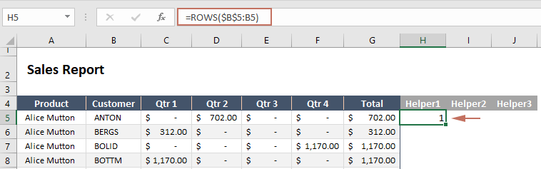
   
3. Dubbelklik op de rechterbenedenhoek van de formulecel, de volgende cel zal automatisch worden gevuld met dezelfde formule.
   
4. Voer in de cel (I5) onder de kop van de tweede hulpcolumnen de volgende formule in en druk op "Enter". Dubbelklik vervolgens op de rechterbenedenhoek van de formulecel om de cellen eronder automatisch te vullen met dezelfde formule.

   =IF(ISNUMBER(SEARCH($M$2,B5)),H5,"")

   Hier is "M2" de cel die is gekoppeld aan de keuzelijst.
   
5. Voer in de cel (J5) onder de kop van de derde hulpcolumnen de volgende formule in en druk op "Enter". Dubbelklik vervolgens op de rechterbenedenhoek van de formulecel om de cellen eronder automatisch te vullen met dezelfde formule.

   =IFERROR(SMALL($I$5:$I$281,H5),"") 

   
6. Kopieer de originele koprij naar een nieuw gebied. Hier plaats ik de koprij onder het zoekvak.
   
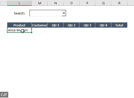
7. Selecteer de cel onder de eerste kop (bijv. L5 in dit voorbeeld), voer de volgende formule in en druk op de "Enter"-toets.

   =IFERROR(INDEX($A$5:$G$281,$J5,COLUMNS($L$4:L4)),"")

   Hier is "A5:G281" het hele gegevensbereik dat u wilt weergeven in de resultaatcel.
   
8. Selecteer deze formulecel, sleep de "Fill Handle" naar rechts en vervolgens naar beneden om de formule toe te passen op de bijbehorende kolommen en rijen.
   
   Opmerkingen:

   • Omdat er geen invoer is in het zoekvak, zullen de resultaten van de formule de ruwe gegevens tonen.
   • Deze methode is hoofdletterongevoelig, wat betekent dat deze tekst overeenkomt ongeacht of u hoofdletters of kleine letters typt.

Resultaat

Laten we nu het zoekvak testen. In dit voorbeeld, wanneer ik een klantennaam invoer of selecteer uit de keuzelijst, worden de bijbehorende rijen die die klantennaam in kolom B bevatten, gefilterd en onmiddellijk weergegeven in het resultaatbereik.

Het maken van een zoekvak in Excel kan aanzienlijk verbeteren hoe u interacteert met uw gegevens, waardoor uw spreadsheets dynamischer en gebruikersvriendelijker worden. Of u nu kiest voor de eenvoud van de FILTER-functie, de visuele ondersteuning van Voorwaardelijke opmaak of de veelzijdigheid van formulecombinaties, elke methode biedt waardevolle tools om uw gegevensmanipulatiecapaciteiten te verbeteren. Experimenteer met deze technieken om te ontdekken welke het beste werkt voor uw specifieke behoeften en gegevensscenario's. Voor wie graag dieper wil duiken in de mogelijkheden van Excel, onze website heeft een schat aan tutorials. Ontdek hier meer Excel-tips en -trucs.

Gerelateerde artikelen