Ga naar hoofdinhoud

Hoe optellen op basis van kolom- en rijcriteria in Excel? 
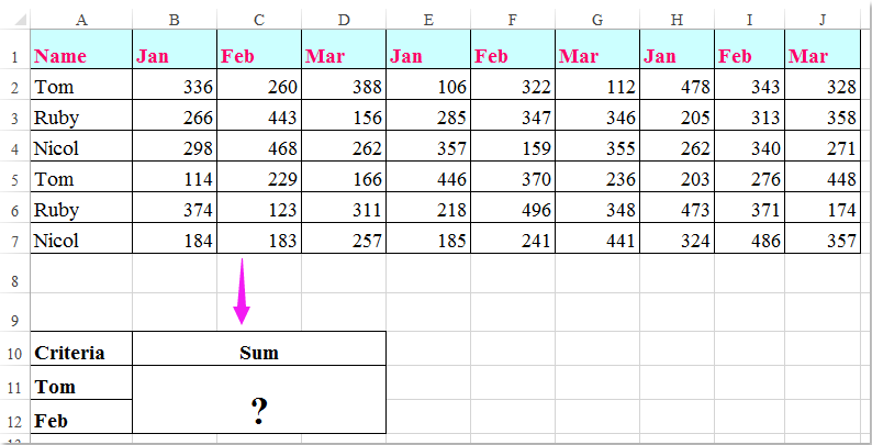
Ik heb een gegevensbereik dat rij- en kolomkoppen bevat, nu wil ik een som nemen van de cellen die voldoen aan zowel de criteria voor kolom- als rijkoppen. Om bijvoorbeeld de cellen bij elkaar op te tellen, is het kolomcriterium Tom en het rijcriterium Feb zoals in het volgende screenshot. In dit artikel zal ik enkele handige formules bespreken om het op te lossen.

criteria voor de rij van de kolommen van documenten 1

Somcellen op basis van kolom- en rijcriteria met formules


pijl blauw rechts bel Somcellen op basis van kolom- en rijcriteria met formules

Hier kunt u de volgende formules toepassen om de cellen op te tellen op basis van zowel de kolom- als de rijcriteria, doe dit als volgt:

Voer een van de onderstaande formules in een lege cel in waarin u het resultaat wilt uitvoeren:

=SUMPRODUCT((A2:A7="Tom")*(B1:J1="Feb")*(B2:J7))

=SUM(IF(B1:J1="Feb",IF(A2:A7="Tom",B2:J7)))

En druk vervolgens op Shift+Ctrl+Enter toetsen samen om het resultaat te krijgen, zie screenshot:
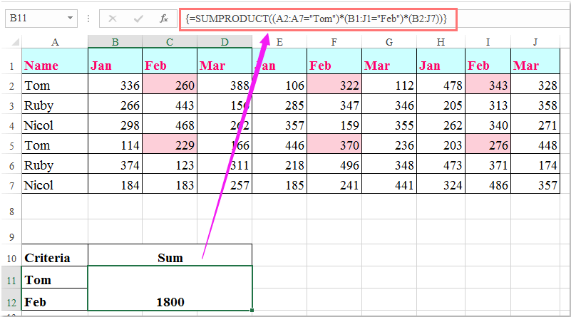
criteria voor de rij van de kolommen van documenten 2

Note: In de bovenstaande formules: Tom en Feb zijn de kolom- en rijcriteria die zijn gebaseerd op, A2: A7, B1: J1 bevatten de kolomkoppen en rijkoppen de criteria, B2: J7 is het gegevensbereik dat u wilt optellen.

Beste Office-productiviteitstools

馃 Kutools AI-assistent: Een revolutie teweegbrengen in de data-analyse op basis van: Intelligente uitvoering   |  Genereer code  |  Aangepaste formules maken  |  Analyseer gegevens en genereer grafieken  |  Roep Kutools-functies aan...
Populaire functies: Zoek, markeer of identificeer duplicaten   |  Verwijder lege rijen   |  Combineer kolommen of cellen zonder gegevens te verliezen   |   Ronde zonder formule ...
Super opzoeken: Meerdere criteria VLookup    VLookup met meerdere waarden  |   VOpzoeken over meerdere bladen   |   Fuzzy opzoeken ....
Geavanceerde vervolgkeuzelijst: Maak snel een vervolgkeuzelijst   |  Afhankelijke vervolgkeuzelijst   |  Multi-select vervolgkeuzelijst ....
Kolom Beheerder: Voeg een specifiek aantal kolommen toe  |  Kolommen verplaatsen  |  Schakel de zichtbaarheidsstatus van verborgen kolommen in  |  Vergelijk bereiken en kolommen ...
Uitgelichte functies: Raster focus   |  Ontwerpweergave   |   Grote formulebalk    Werkmap- en bladbeheer   |  resource Library (Auto-tekst)   |  Datumkiezer   |  Combineer werkbladen   |  Cellen coderen/decoderen    Stuur e-mails per lijst   |  Super filter   |   Speciaal filter (filter vet/cursief/doorhalen...) ...
Top 15 gereedschapsets12 Tekst Tools (toe te voegen tekst, Tekens verwijderen, ...)   |   50+ tabel Types (Gantt Chart, ...)   |   40+ Praktisch Formules (Bereken leeftijd op basis van verjaardag, ...)   |   19 Invoeging Tools (QR-code invoegen, Afbeelding invoegen vanaf pad, ...)   |   12 Camper ombouw Tools (Getallen naar woorden, Currency Conversion, ...)   |   7 Samenvoegen en splitsen Tools (Geavanceerd Combineer rijen, Gespleten cellen, ...)   |   ... en meer

Geef uw Excel-vaardigheden een boost met Kutools voor Excel en ervaar effici毛ntie als nooit tevoren. Kutools voor Excel biedt meer dan 300 geavanceerde functies om de productiviteit te verhogen en tijd te besparen.  Klik hier om de functie te krijgen die u het meest nodig heeft...

Omschrijving


Office-tabblad Brengt een interface met tabbladen naar Office en maakt uw werk veel gemakkelijker

  • Schakel bewerken en lezen met tabbladen in Word, Excel, PowerPoint in, Publisher, Access, Visio en Project.
  • Open en maak meerdere documenten in nieuwe tabbladen van hetzelfde venster in plaats van in nieuwe vensters.
  • Verhoogt uw productiviteit met 50% en vermindert honderden muisklikken voor u elke dag!
Comments (16)
No ratings yet. Be the first to rate!
This comment was minimized by the moderator on the site
My data that I am trying to retrieve is in a table. Would this impact the result at all? I have:

=SUM(IF('[Primary Controller Active Project Database (KC notes)1.xlsx]Active Project Tracking'!$B2:$B66=X2,IF('[Primary Controller Active Project Database (KC notes)1.xlsx]Active Project Tracking'!$A1:$AV1=AH10,'[Primary Controller Active Project Database (KC notes)1.xlsx]Active Project Tracking'!$H$2:$AV$66)))

So I think the equivalent would be if you did your information above, but in a table in a different workbook. Thoughts?
This comment was minimized by the moderator on the site
If there were negatives in the matrix and you only wanted to include the positives, what would you do? 
I tried to do something like this:

=SUMPRODUCT((Column = Criteria)* ( Row = Criteria) * (second column = Criteria) * (Matrix) * (Matrix >0))

This comment was minimized by the moderator on the site
Is there a way to do this but instead of writing "Tom" & "Feb" in the formula, you are able to reference the criteria cells e.g.A11 & A12?
This comment was minimized by the moderator on the site
Hello, Rianna,Yest, as you said, you can use the cell references to replace the text in the formula, such as:
=SUMPRODUCT((A2:A7=A2)*(B1:J1=C1)*(B2:J7))
=SUM(IF(B1:J1=C1,IF(A2:A7=A2,B2:J7)))
This comment was minimized by the moderator on the site
In the above example which formula should I use if I wanted calculate the sum of the amounts earned by Tom Ruby & Nicol in March?
This comment was minimized by the moderator on the site
Hello, Nabar,To get the result you want, please apply the below formula:=SUMPRODUCT(((A2:A7="Tom")+(A2:A7="Nicol")+(A2:A7="Ruby"))*(B1:J1="Mar")*(B2:J7))
Please try, hope it can help you!
This comment was minimized by the moderator on the site
Hello Skyyang,
Thank you for your response. I tried the formula you suggested but I am not getting the right answer. Probably I wasn't able to put my query correctly. Let me try again I have a spreadsheet with data with daily calculation, I have numbered the first row 1,2,3,4.....132. 2nd, 3rd 4th &5th rows has table headings. The first column has line no's numbered 1, 2,3,.....3005 starting from row 6,range B6:EF3005 has data filled in on everyday basis. In second sheet i have a table in which I want to apply a formula which will look up two line numbers fed in two different rows and calculate the sum from the range B6: EF3005 from the data spreadsheet between the two line numbers from a certain column viz sum of values in column 15 between rows (line No's) 50 & 85.
This comment was minimized by the moderator on the site
Is there a way to make this work with wildcard characters? I'd like to use it on everything starting with certain characters, but with (a fixed number of) undefined characters at the end, i.e. =SUM(IF(B1:J1="Fe*",IF(A2:A7="To*",B2:J7)))
This comment was minimized by the moderator on the site
Should anyone have the same question, this is how I solved it (in Google Sheets, not tested in Excel):

=ArrayFormula(SUM(IF(regexmatch(O5:W5,"^Fe."),IF(regexmatch(N6:N11,"^To."),O6:W11))))

Note that the IF function does not support wildcard characters and that for regexmatch the wildcards are different and can be found here: https://github.com/google/re2/blob/master/doc/syntax.txt
In this particular instance, I used ^ to indicate that Fe & Tom occur at the beginning of text and . to allow for any following character (* would mean zero or more of the previous character, e.g. Fe* would only look for instances with 1 or more "e"s after F)
This comment was minimized by the moderator on the site
I tried to create a formula to calculate if the D12 is blank, it will calculate from K12 to AH12 but it seems this part ' regexmatch(D12,"")' is not working
ArrayFormula(SUM(IF(regexmatch(D12,""),K12:AH12)))
This comment was minimized by the moderator on the site
Thank you so much! You made my day!! @TeSageDS
This comment was minimized by the moderator on the site
how would you do this same formula if you wanted to sum both Feb and March together? please help! thanks

=SUMPRODUCT((A2:A7="Tom")*(B1:J1="Feb")*(B2:J7))
This comment was minimized by the moderator on the site
Hello,Angela,
To solve your problem, you just need to apply the below formula, please try it.

=SUMPRODUCT((A2:A7="Tom")*((B1:J1="Feb")+(B1:J1="Mar"))*(B2:J7)).

Hope it can help you!
This comment was minimized by the moderator on the site
Brilliant
This comment was minimized by the moderator on the site
Worth pointing out that of the two formulas provided above you do not need to enter the SUMPRODUCT formula with Ctrl + Shift + Enter. It will work perfectly well without it.
This comment was minimized by the moderator on the site
Awesome, this is the one what i was looking for. thanks for the help
There are no comments posted here yet
Please leave your comments in English
Posting as Guest
Rate this post:
0   Characters
Suggested Locations