Ga naar hoofdinhoud

Hoe vind je de zoveelste niet-lege cel in Excel?

Hoe kon je de n-de niet-lege celwaarde uit een kolom of rij in Excel vinden en retourneren? In dit artikel zal ik het hebben over enkele nuttige formules waarmee u deze taak kunt oplossen.

Zoek en retourneer de n-de niet-lege celwaarde uit een kolom met formule

Zoek en retourneer de n-de niet-lege celwaarde uit een rij met formule


pijl blauw rechts bel Zoek en retourneer de n-de niet-lege celwaarde uit een kolom met formule

Ik heb bijvoorbeeld een kolom met gegevens zoals in het volgende screenshot wordt getoond, nu krijg ik de derde niet-lege celwaarde uit deze lijst.

doc zoek n-de niet-blanco 1

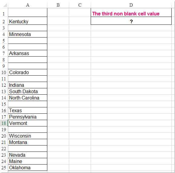
Voer deze formule in: =INDEX($A$1:$A$25,SMALL(ROW($A$1:$A$25)+(100*($A$1:$A$25="")), 3))&"" in een lege cel waar u het resultaat wilt uitvoeren, bijvoorbeeld D2, en druk vervolgens op Ctrl + Shift + Enter toetsen samen om het juiste resultaat te krijgen, zie screenshot:

doc zoek n-de niet-blanco 2

Note: In bovenstaande formule, A1: A25 is de datalijst die u wilt gebruiken, en het nummer 3 geeft de derde niet-lege celwaarde aan die u wilt retourneren, als u de tweede niet-lege cel wilt krijgen, hoeft u alleen het nummer 3 in 2 te wijzigen.


pijl blauw rechts bel Zoek en retourneer de n-de niet-lege celwaarde uit een rij met formule

Als u de n-de niet-lege celwaarde op een rij wilt vinden en retourneren, kan de volgende formule u helpen, doe dit als volgt:

Voer deze formule in: =INDEX($A$1:$M$1,SMALL(IF($A$1:$M$1<>"",COLUMN($A$1:$M$1)-COLUMN($A$1)+1),4)) in een lege cel waar u het resultaat wilt zoeken, en druk vervolgens op Ctrl + Shift + Enter toetsen samen om het resultaat te krijgen, zie screenshot:
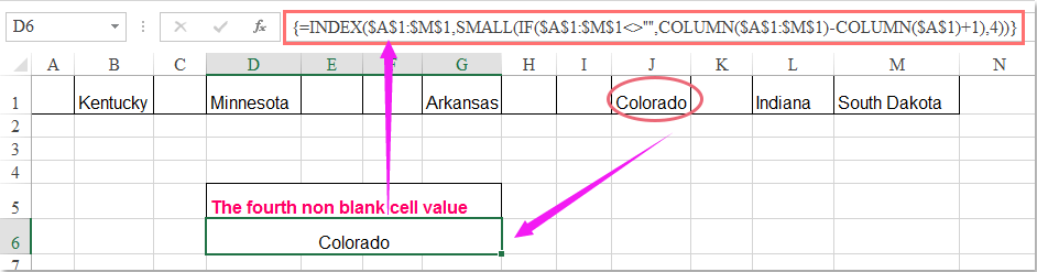
doc zoek n-de niet-blanco 3

Opmerking: In bovenstaande formule, A1: M1 zijn de rijwaarden die u wilt gebruiken, en het nummer 4 is de vierde niet-lege celwaarde die u wilt retourneren, als u de tweede niet-lege cel wilt krijgen, hoeft u alleen het nummer 4 in 2 te wijzigen.

Beste Office-productiviteitstools

馃 Kutools AI-assistent: Een revolutie teweegbrengen in de data-analyse op basis van: Intelligente uitvoering   |  Genereer code  |  Aangepaste formules maken  |  Analyseer gegevens en genereer grafieken  |  Roep Kutools-functies aan...
Populaire functies: Zoek, markeer of identificeer duplicaten   |  Verwijder lege rijen   |  Combineer kolommen of cellen zonder gegevens te verliezen   |   Ronde zonder formule ...
Super opzoeken: Meerdere criteria VLookup    VLookup met meerdere waarden  |   VOpzoeken over meerdere bladen   |   Fuzzy opzoeken ....
Geavanceerde vervolgkeuzelijst: Maak snel een vervolgkeuzelijst   |  Afhankelijke vervolgkeuzelijst   |  Multi-select vervolgkeuzelijst ....
Kolom Beheerder: Voeg een specifiek aantal kolommen toe  |  Kolommen verplaatsen  |  Schakel de zichtbaarheidsstatus van verborgen kolommen in  |  Vergelijk bereiken en kolommen ...
Uitgelichte functies: Raster focus   |  Ontwerpweergave   |   Grote formulebalk    Werkmap- en bladbeheer   |  resource Library (Auto-tekst)   |  Datumkiezer   |  Combineer werkbladen   |  Cellen coderen/decoderen    Stuur e-mails per lijst   |  Super filter   |   Speciaal filter (filter vet/cursief/doorhalen...) ...
Top 15 gereedschapsets12 Tekst Tools (toe te voegen tekst, Tekens verwijderen, ...)   |   50+ tabel Types (Gantt Chart, ...)   |   40+ Praktisch Formules (Bereken leeftijd op basis van verjaardag, ...)   |   19 Invoeging Tools (QR-code invoegen, Afbeelding invoegen vanaf pad, ...)   |   12 Camper ombouw Tools (Getallen naar woorden, Currency Conversion, ...)   |   7 Samenvoegen en splitsen Tools (Geavanceerd Combineer rijen, Gespleten cellen, ...)   |   ... en meer

Geef uw Excel-vaardigheden een boost met Kutools voor Excel en ervaar effici毛ntie als nooit tevoren. Kutools voor Excel biedt meer dan 300 geavanceerde functies om de productiviteit te verhogen en tijd te besparen.  Klik hier om de functie te krijgen die u het meest nodig heeft...

Omschrijving


Office-tabblad Brengt een interface met tabbladen naar Office en maakt uw werk veel gemakkelijker

  • Schakel bewerken en lezen met tabbladen in Word, Excel, PowerPoint in, Publisher, Access, Visio en Project.
  • Open en maak meerdere documenten in nieuwe tabbladen van hetzelfde venster in plaats van in nieuwe vensters.
  • Verhoogt uw productiviteit met 50% en vermindert honderden muisklikken voor u elke dag!
Comments (10)
No ratings yet. Be the first to rate!
This comment was minimized by the moderator on the site
CIAO STO CERCANDO DI APPLICARE LA TUA FORMULA MA NON MI FUNZIONA, DOVE STO SBAGLIANDO?
=INDICE($K$37:$K$88;MIN(RIGHE($K$37:$K$88)+RIGHE(100*($K$37:$K$88=""));6))&""
DEVO VISUALIZZARE L'ENNESIMA RIGA DIVERSA DA VUOTO

GRAzie
This comment was minimized by the moderator on the site
=INDICE($K$37:$K$88;MIN(RIGHE($K$37:$K$88)+(100*($K$37:$K$88=""));6))&""
This comment was minimized by the moderator on the site
I'm running this formula on a ~400 row sheet with around 20 blanks mixed throughout the data, and it's working perfectly EXCEPT when I fill the series down, it sometimes duplicates a row for some reason. For example, it seems to think a value is somehow simultaneously the 331st non-blank and the 332nd.

Things I've noticed:
-Duplications always happen in pairs (ex. 331 and 332 are duplicates, 333 and 334 will also be), then it goes back to normal for a while.
-Raw data also has blanks in pairs, but not corresponding to the duplicates
-No duplications occur in the first 94 rows, but they happen every 33-35 rows after that
-Does not appear to be linked to the value in the cell being duplicated
-I have entered as an array and as a standard formula, no difference in function

For reference, here's my actual formula:

=INDEX('PO Raw Data'!CR:CR,SMALL(ROW('PO Raw Data'!CR:CR)+(100*('PO Raw Data'!CR:CR="")),$W2)&"")

Note $W2 refers to a helper column and counts up as the data set is filled down, but only because I couldn't get it to count up when I just used a number instead of cell reference.
When I've replaced that cell reference (ex. $W2) with the appropriate number, same result.


Any thoughts on what I can do to fix that?
This comment was minimized by the moderator on the site
very helpful,
although when I return the nth non blank cell in a column set to DATE, the returned value appears as number(general number).formatting the cell into DATE also doesn't change the result. could you please give me a hand!
thanks a lot
This comment was minimized by the moderator on the site
Hello, Shirazi,
Sorry, maybe there is no direct formula for you to get the date format.

If someone else has the solution, please comment here.
This comment was minimized by the moderator on the site
Hi everyone!


Could you also help me return the row number of the second, third non-blank cell?


Please help me.
This comment was minimized by the moderator on the site
Hello, John,
the following formula can help you to get all the row numbers of the non-blank cells, please try it, thank you!
=IFERROR(ROW(INDEX($A$1:$A$12,SMALL(INDEX(NOT(ISBLANK($A$1:$A$12))*ROW($A$1:$A$12),0),COUNTBLANK($A$1:$A$12)+ROW(A1)))),"")
This comment was minimized by the moderator on the site
Hey everyone,

I have a table with numerous columns and rows. The rows have range names, and a description/location at the beginning of the row range with its own range, example "Building No.s". There are multiple Row Ranges/ Buildings. There are headers at the top of each columns for specific "Building Assembly Types". The table content is numeric quantities for each type "Building Assembly Type" for each specific "Building" description/location. There could be as many as (100) "Building Assembly Types" column headers but I will limit the assemblies to (10) per row range, so there will be numerous blank cells in each "Building No." range.

I have other summary tables set up for each "Building" that I want to pull the non-blank cells quantities to, along with the corresponding header "Assembly Type" for each "Building" with a (10) max "Assemblies" per page.

I can identify the non-blank cell quantities by use of the array formula above for rows. The problem I am having is identifying the header that corresponds to it.

Ultimately if I can identify the "Assembly" header, I can always index the "Quantities" once I have the header "Assembly" identified for each "Building". Then I would be able do a lookup for all the parts associated with each "Assembly" type for that "Building" from my Assembly parts database and multiply it times the "Quantity" of each assembly type.

Hopefully this makes since and someone can help.
This comment was minimized by the moderator on the site
Hello, I am looking for the third blank row in a column and I copied your formula and just changed the range from $A$1:$A:$25 to my range $D$306:$D$354. But when I change the range I get #REF! as my answer. I already converted to an array, control-shift-enter. Now the cell range I am referencing has formulas in them, so could that be why I am getting #REF. Your formula: =INDEX($A$1:$A$25,SMALL(ROW($A$1:$A$25)+(100*($A$1:$A$25="")), 3))&"" My formula: =INDEX($D$306:$D$354,SMALL(ROW($D$306:$D$354)+(1*($D$306:$D$354="")), 2))&"" Thanks, Noel
This comment was minimized by the moderator on the site
you have put the 1 instead of 100 therefore answered was wrong. please use below formula

INDEX($D$306:$D$354,SMALL(ROW($D$306:$D$354)+(100*($D$306:$D$354="")), 3))&"" than ctrl + shift+enter
There are no comments posted here yet
Please leave your comments in English
Posting as Guest
Rate this post:
0   Characters
Suggested Locations