Hoe het eerste niet-nulwaarde opzoeken en de bijbehorende kolomkop retourneren in Excel?
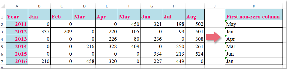
Bij het werken met gegevens in Excel is het gebruikelijk om de positie van de eerste niet-nulwaarde binnen een rij te identificeren en de bijbehorende kolomkop weer te geven. Bijvoorbeeld, in een dataset waar elke rij een ander item of persoon vertegenwoordigt en kolommen tijdperken of categorieën vertegenwoordigen, zou je willen weten wanneer een waarde voor het eerst verschijnt voor elke rij. Handmatig elke rij controleren op de eerste niet-nulwaarde kan tijdrovend zijn, vooral naarmate de gegevensgrootte groeit. Het automatiseren van dit zoekproces verbetert niet alleen de efficiëntie, maar vermindert ook fouten, waardoor je analyses betrouwbaarder worden. Dit artikel legt meerdere praktische manieren uit om dit doel te bereiken, van het gebruik van veelzijdige Excel-formules tot het toepassen van VBA-macros die vooral nuttig zijn voor grote datasets of terugkerende rapporten.
- Zoek de eerste niet-nulwaarde en retourneer de bijbehorende kolomkop met een formule
- Gebruik een VBA-macro om de kolomkop van de eerste niet-nulwaarde in elke rij te vinden en retourneren
 Zoek de eerste niet-nulwaarde en retourneer de bijbehorende kolomkop met een formule
Om efficiënt de kolomkop in een bepaalde rij te identificeren waar de eerste niet-nulwaarde verschijnt, kun je een ingebouwde Excel-formule gebruiken. Deze aanpak is vooral geschikt voor kleine tot middelgrote datasets waar real-time herberekening en eenvoudige instelling belangrijk zijn.
1. Selecteer een lege cel om het resultaat weer te geven; in dit voorbeeld wordt cel K2 gebruikt.
=INDEX($B$1:$I$1,MATCH(TRUE,INDEX(B2:I2<>0,),0))2. Nadat je de formule hebt ingevoerd, druk op Enter om te bevestigen. Selecteer vervolgens K2 en gebruik de vulgreep om de formule naar beneden te slepen om deze toe te passen op de rest van de rijen indien nodig.
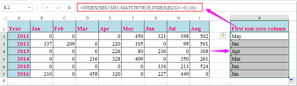
Opmerking: In de bovenstaande formule verwijst B1:I1 naar het bereik van kolomkoppen dat je wilt retourneren, en B2:I2 is de rijgegevens die je analyseert op de eerste niet-nulwaarde.
Als je gegevens in verschillende kolommen of rijen begint, vergeet dan niet de formulebereiken dienovereenkomstig aan te passen. Ook werkt deze formule effectief zolang er ten minste één niet-nulwaarde in elke geanalyseerde rij is; als alle waarden nul zijn, zal de formule een fout retourneren. In dergelijke gevallen kun je overwegen de formule in IFERROR te verpakken zoals deze: =IFERROR(INDEX($B$1:$I$1,MATCH(TRUE,INDEX(B2:I2<>0,),0)),"Geen niet-nul") om een aangepast bericht in plaats van een fout te retourneren.
Deze op formules gebaseerde oplossing is ideaal wanneer je dynamische, direct bijwerkende resultaten wilt terwijl je invoergegevens veranderen. Echter, voor extreem grote datasets kan de berekeningsnelheid worden beïnvloed, en je zou kunnen zoeken naar een VBA-aanpak om workflowautomatisering te verbeteren of handmatige operaties te verminderen.
Gebruik een VBA-macro om de kolomkop van de eerste niet-nulwaarde in elke rij te vinden en retourneren
Als je vaak deze zoektaak moet uitvoeren over veel rijen of op grote datasets, of als je het proces wilt automatiseren voor efficiëntie, is het gebruik van een VBA-macro een praktische alternatief. Deze methode is vooral voordelig voor periodieke rapportgeneratie of wanneer je gegevenstabellen behandelt die vaak in grootte veranderen. De macro zal elke gespecificeerde rij doorzoeken voor de eerste niet-nulwaarde en de bijbehorende kolomkop retourneren naar een doelcel.
1. Klik op het tabblad Ontwikkelaar > Visual Basic om het Microsoft Visual Basic for Applications-venster te openen. (Als het tabblad Ontwikkelaar niet zichtbaar is, kun je het toevoegen via Bestand > Opties > Aanpassen Lint.) Klik in de VBA-editor op Invoegen > Module.
2. Kopieer en plak de volgende VBA-code in de nieuwe module:
Sub LookupFirstNonZeroAndReturnHeader()
    Dim ws As Worksheet
    Dim dataRange As Range
    Dim headerRange As Range
    Dim outputCell As Range
    Dim r As Range
    Dim c As Range
    Dim firstNonZeroCol As Integer
    Dim i As Long
    Dim xTitleId As String
    On Error Resume Next
    xTitleId = "KutoolsforExcel"
    Set ws = Application.ActiveSheet
    Set dataRange = Application.InputBox("Select the data range (excluding headers):", xTitleId, Selection.Address, Type:=8)
    If dataRange Is Nothing Then Exit Sub
    Set headerRange = ws.Range(dataRange.Offset(-1, 0).Resize(1, dataRange.Columns.Count).Address)
    For i = 1 To dataRange.Rows.Count
        Set r = dataRange.Rows(i)
        firstNonZeroCol = 0

        For Each c In r.Columns
            If c.Value <> 0 And c.Value <> "" Then
                firstNonZeroCol = c.Column - dataRange.Columns(1).Column + 1
                Exit For
            End If
        Next c

        Set outputCell = r.Cells(1, r.Columns.Count + 1)

        If firstNonZeroCol > 0 Then
            outputCell.Value = headerRange.Cells(1, firstNonZeroCol).Value
        Else
            outputCell.Value = "No non-zero"
        End If
    Next i

    On Error GoTo 0
    MsgBox "Completed! Results are in the column to the right of your data.", vbInformation, "KutoolsforExcel"
End Sub
3. Om de macro uit te voeren, klik op de knop Uitvoeren of druk op de F5-toets. Een dialoogvenster vraagt je om het gegevensbereik te selecteren (exclusief de kolomkoppen). Nadat de macro is uitgevoerd, wordt de kolom onmiddellijk rechts van het geselecteerde gegevensgebied gevuld met de kop van de eerste niet-nulwaarde voor elke rij, of een "Geen niet-nul"-bericht als geen niet-nulwaarde wordt gevonden.
Deze VBA-aanpak excelleert in herhalende taken en is uitstekend geschikt voor het verwerken van grote datasets, waardoor handmatige inspanningen worden verminderd. Zorg er echter voor dat macros zijn ingeschakeld in uw Excel-omgeving en maak altijd een back-up van uw werkmap voordat u code uitvoert.
Opmerking: Als u fouten tegenkomt, controleer dan of uw selectie de koprij uitsluit en alleen de gegevensrijen omvat.

Ontdek de Magie van Excel met Kutools AI
- Slimme Uitvoering: Voer celbewerkingen uit, analyseer gegevens en maak diagrammen – allemaal aangestuurd door eenvoudige commando's.
- Aangepaste Formules: Genereer op maat gemaakte formules om uw workflows te versnellen.
- VBA-codering: Schrijf en implementeer VBA-code moeiteloos.
- Formule-uitleg: Begrijp complexe formules gemakkelijk.
- Tekstvertaling: Overbrug taalbarrières binnen uw spreadsheets.
Beste productiviteitstools voor Office
Verbeter je Excel-vaardigheden met Kutools voor Excel en ervaar ongeëvenaarde efficiëntie. Kutools voor Excel biedt meer dan300 geavanceerde functies om je productiviteit te verhogen en tijd te besparen. Klik hier om de functie te kiezen die je het meest nodig hebt...
Office Tab brengt een tabbladinterface naar Office en maakt je werk veel eenvoudiger
- Activeer tabbladbewerking en -lezen in Word, Excel, PowerPoint, Publisher, Access, Visio en Project.
- Open en maak meerdere documenten in nieuwe tabbladen van hetzelfde venster, in plaats van in nieuwe vensters.
- Verhoog je productiviteit met50% en bespaar dagelijks honderden muisklikken!
Alle Kutools-invoegtoepassingen. Eén installatieprogramma
Kutools for Office-suite bundelt invoegtoepassingen voor Excel, Word, Outlook & PowerPoint plus Office Tab Pro, ideaal voor teams die werken met Office-toepassingen.
- Alles-in-één suite — invoegtoepassingen voor Excel, Word, Outlook & PowerPoint + Office Tab Pro
- Eén installatieprogramma, één licentie — in enkele minuten geïnstalleerd (MSI-ready)
- Werkt beter samen — gestroomlijnde productiviteit over meerdere Office-toepassingen
- 30 dagen volledige proef — geen registratie, geen creditcard nodig
- Beste prijs — bespaar ten opzichte van losse aanschaf van invoegtoepassingen