Unieke waarden extraheren op basis van één of meerdere criteria in Excel
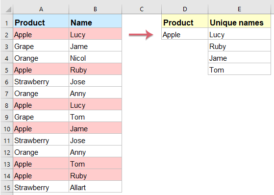
Het extraheren van unieke waarden op basis van criteria is een cruciale taak voor data-analyse en rapportage. Stel dat je het gegevensbereik aan de linkerkant hebt, en je wilt alleen de unieke namen in kolom B weergeven op basis van een specifiek criterium in kolom A. Of je nu werkt met oudere versies van Excel of gebruik maakt van de nieuwste functies in Excel 365/2021, deze handleiding laat je zien hoe je unieke waarden efficiënt kunt extraheren.
Unieke waarden extraheren op basis van criteria in Excel
Unieke waarden extraheren op basis van meerdere criteria in Excel
Unieke waarden extraheren uit een lijst met cellen met Kutools voor Excel
Unieke waarden extraheren op basis van criteria in Excel
• Met arrayformule om de unieke waarden verticaal weer te geven
Om dit probleem op te lossen, kun je een complexe arrayformule toepassen. Volg de volgende stappen:
1. Voer de onderstaande formule in een lege cel in waar je de extractieresultaten wilt weergeven. In dit voorbeeld plaats ik het in cel E2, en druk vervolgens op Shift + Ctrl + Enter om de eerste unieke waarde te krijgen.
=IFERROR(INDEX($B$2:$B$15, MATCH(0, IF($D$2=$A$2:$A$15, COUNTIF($E$1:$E1, $B$2:$B$15), ""), 0)),"")2. Sleep daarna de vulgreep naar beneden tot er lege cellen verschijnen, en nu zijn alle unieke waarden op basis van het specifieke criterium weergegeven, zie screenshot:

• Unieke waarden extraheren en weergeven in één cel met Kutools voor Excel
Kutools voor Excel biedt een eenvoudige manier om unieke waarden te extraheren en ze in één cel weer te geven, wat tijd en moeite bespaart bij het werken met grote datasets zonder dat je formules hoeft te onthouden.
Nadat je Kutools voor Excel hebt geïnstalleerd, doe dan het volgende:
Klik op "Kutools" > "Super ZOEKEN" > "Eén-op-veel-zoeken (retourneert meerdere resultaten)" om het dialoogvenster te openen. Specificeer in het dialoogvenster de bewerkingen als volgt:
- Selecteer het "Plaatsingsgebied lijst" en "Bereik van waarden dat moet worden doorzocht" apart in de tekstvakken;
- Selecteer het tabelbereik dat je wilt gebruiken;
- Specificeer de sleutelkolom en retourkolom afzonderlijk in de vervolgkeuzelijsten "Sleutelkolom" en "Retourkolom";
- Klik ten slotte op de knop OK.


Resultaat:
Alle unieke namen op basis van de criteria zijn geëxtraheerd in één cel, zie screenshot:
• Met formule in Excel 365, Excel 2021 en latere versies om unieke waarden verticaal weer te geven
Met Excel 365 en Excel 2021 maken functies zoals UNIEK en FILTER het extraheren van unieke waarden eenvoudiger.
Voer de onderstaande formule in een lege cel in, en druk vervolgens op Enter om alle unieke namen tegelijkertijd verticaal te krijgen.
=UNIQUE(FILTER(B2:B15, A2:A15=D2))
- FILTER(B2:B15, A2:A15=D2):
- FILTER: Filtert gegevens uit B2:B15.
- A2:A15=D2: Controleert waar de waarden in A2:A15 overeenkomen met de waarde in D2. Alleen rijen die aan deze voorwaarde voldoen, worden opgenomen in het resultaat.
- UNIEK(...):
Zorgt ervoor dat alleen unieke waarden uit de gefilterde resultaten worden geretourneerd.
Unieke waarden extraheren op basis van meerdere criteria in Excel
• Met arrayformule om de unieke waarden verticaal weer te geven
Als je de unieke waarden wilt extraheren op basis van twee voorwaarden, is hier nog een andere arrayformule die je kan helpen. Doe het volgende:
1. Voer de onderstaande formule in een lege cel in waar je de unieke waarden wilt weergeven. In dit voorbeeld plaats ik het in cel G2, en druk vervolgens op Shift + Ctrl + Enter om de eerste unieke waarde te krijgen.
=IFERROR(INDEX($C$2:$C$15,MATCH(0,COUNTIF(G1:$G$1,$C$2:$C$15)+IF($A$2:$A$15<>$E$2,1,0)+IF($B$2:$B$15<>$F$2,1,0),0)),"")2. Sleep daarna de vulgreep naar beneden tot er lege cellen verschijnen, en nu zijn alle unieke waarden op basis van de specifieke twee voorwaarden weergegeven, zie screenshot:

• Met in Excel 365, Excel 2021 en latere versies om unieke waarden verticaal weer te geven
Voor nieuwere Excel-versies is het extraheren van unieke waarden op basis van meerdere criteria veel eenvoudiger.
Voer de onderstaande formule in een lege cel in, en druk vervolgens op Enter om alle unieke namen tegelijkertijd verticaal te krijgen.
=UNIQUE(FILTER(C2:C15, (A2:A15=E2) * (B2:B15=F2)))
- FILTER(C2:C15, (A2:A15=E2) * (B2:B15=F2)):
- FILTER: Filtert gegevens uit C2:C15.
- (A2:A15=E2): Controleert of de waarden in kolom A overeenkomen met de waarde in E2.
- (B2:B15=F2): Controleert of de waarden in kolom B overeenkomen met de waarde in F2.
- *: Combineert de twee voorwaarden met EN-logica, wat betekent dat beide voorwaarden waar moeten zijn om een rij op te nemen.
- UNIEK(...):
Verwijdert dubbele waarden uit de gefilterde resultaten, zodat de uitkomst alleen unieke waarden bevat.
Unieke waarden extraheren uit een lijst met cellen met Kutools voor Excel
Soms wil je misschien unieke waarden extraheren uit een lijst met cellen. Hier raad ik een handig hulpmiddel aan, Kutools voor Excel. De functie "Unieke cellen in een bereik extraheren (inclusief de eerste duplicatie)" stelt je in staat om snel unieke waarden te extraheren.
1. Klik op een cel waar je het resultaat wilt weergeven. (Opmerking: Selecteer geen cel in de eerste rij.)
2. Klik vervolgens op "Kutools" > "Formulehulp" > "Formulehulp", zie screenshot:

3. Voer in het dialoogvenster "Formulehulp" de volgende bewerkingen uit:
- Selecteer de optie "Tekst" in de vervolgkeuzelijst "Formuletype";
- Kies vervolgens "Unieke cellen in een bereik extraheren (inclusief de eerste duplicatie)" in de lijst met formules;
- Selecteer in het rechtergedeelte "Argumentinvoer" een lijst met cellen waaruit je unieke waarden wilt extraheren.

4. Klik vervolgens op de knop Ok. Het eerste resultaat wordt weergegeven in de cel. Selecteer de cel en sleep de vulgreep over de cellen waarin je alle unieke waarden wilt weergeven tot er lege cellen verschijnen, zie screenshot:

Het extraheren van unieke waarden op basis van criteria in Excel is een essentiële taak voor efficiënte data-analyse, en Excel biedt meerdere manieren om dit te bereiken op basis van je versie en behoeften. Door de juiste methode te kiezen voor je versie van Excel en je specifieke vereisten, kun je unieke waarden efficiënt extraheren. Als je meer Excel-tips en -trucs wilt ontdekken, onze website biedt duizenden tutorials.
Meer gerelateerde artikelen:
- Tel het aantal unieke en verschillende waarden uit een lijst
- Stel dat je een lange lijst met waarden hebt met enkele dubbele items, en nu wil je het aantal unieke waarden tellen (de waarden die maar één keer in de lijst voorkomen) of verschillende waarden (alle verschillende waarden in de lijst, wat betekent unieke waarden + eerste duplicaatwaarden) in een kolom zoals links in de schermafbeelding te zien is. In dit artikel zal ik bespreken hoe je deze taak in Excel kunt aanpakken.
- Som unieke waarden op basis van criteria in Excel
- Bijvoorbeeld, ik heb een bereik met gegevens dat kolommen Naam en Bestelling bevat, en nu wil ik alleen unieke waarden in de kolom Bestelling optellen op basis van de kolom Naam zoals in de volgende schermafbeelding te zien is. Hoe los je deze taak snel en gemakkelijk op in Excel?
- Transponeer cellen in één kolom op basis van unieke waarden in een andere kolom
- Stel dat je een bereik met gegevens hebt dat twee kolommen bevat, en nu wil je cellen in één kolom transponeren naar horizontale rijen op basis van unieke waarden in een andere kolom om het volgende resultaat te krijgen. Heb je goede ideeën om dit probleem in Excel op te lossen?
- Unieke waarden samenvoegen in Excel
- Als ik een lange lijst met waarden heb die gevuld is met enkele dubbele gegevens, wil ik nu alleen de unieke waarden vinden en deze samenvoegen in één cel. Hoe kan ik dit probleem snel en gemakkelijk in Excel oplossen?
Beste productiviteitstools voor Office
Verbeter je Excel-vaardigheden met Kutools voor Excel en ervaar ongeëvenaarde efficiëntie. Kutools voor Excel biedt meer dan300 geavanceerde functies om je productiviteit te verhogen en tijd te besparen. Klik hier om de functie te kiezen die je het meest nodig hebt...
Office Tab brengt een tabbladinterface naar Office en maakt je werk veel eenvoudiger
- Activeer tabbladbewerking en -lezen in Word, Excel, PowerPoint, Publisher, Access, Visio en Project.
- Open en maak meerdere documenten in nieuwe tabbladen van hetzelfde venster, in plaats van in nieuwe vensters.
- Verhoog je productiviteit met50% en bespaar dagelijks honderden muisklikken!
Alle Kutools-invoegtoepassingen. Eén installatieprogramma
Kutools for Office-suite bundelt invoegtoepassingen voor Excel, Word, Outlook & PowerPoint plus Office Tab Pro, ideaal voor teams die werken met Office-toepassingen.
- Alles-in-één suite — invoegtoepassingen voor Excel, Word, Outlook & PowerPoint + Office Tab Pro
- Eén installatieprogramma, één licentie — in enkele minuten geïnstalleerd (MSI-ready)
- Werkt beter samen — gestroomlijnde productiviteit over meerdere Office-toepassingen
- 30 dagen volledige proef — geen registratie, geen creditcard nodig
- Beste prijs — bespaar ten opzichte van losse aanschaf van invoegtoepassingen