Hoe kan ik in Excel zoeken en meerdere overeenkomstige waarden samenvoegen?
Bij het gebruik van VLOOKUP in Excel zal de functie doorgaans alleen de eerste overeenkomstige waarde retourneren die hij vindt voor een bepaald zoekcriterium. Er zijn echter veel gebruikelijke scenario's waarin je mogelijk alle overeenkomstige waarden die gekoppeld zijn aan een specifieke sleutel moet ophalen en combineren, zoals het weergeven van alle studenten in een klas of alle producten die bij een bepaalde categorie horen. Omdat de standaard VLOOKUP-functie hierin beperkt is, vraag je je misschien af hoe je zowel kunt zoeken als meerdere overeenkomstige resultaten in één cel kunt samenvoegen. Hieronder bekijken we verschillende praktische en efficiënte methoden om deze taak uit te voeren, geschikt voor verschillende Excel-versies en gebruikersvoorkeuren.
Zoek en samenvoegen van meerdere overeenkomstige waarden in Excel
Zoek en samenvoeg meerdere overeenkomstige waarden met TEXTJOIN- en FILTER-functies
Als je Excel 365 of Excel 2021 gebruikt, biedt de combinatie van TEXTJOIN- en FILTER-functies een efficiënte, formulegebaseerde benadering om te zoeken en alle overeenkomstige waarden samen te voegen. Deze oplossing is vooral geschikt voor dynamische en bijgewerkte datasets, omdat deze automatisch het resultaat vernieuwt wanneer de brongegevens veranderen. Het wordt het beste toegepast wanneer jouw versie van Excel de FILTER-functie ondersteunt, wat exclusief is voor recente Office-versies.
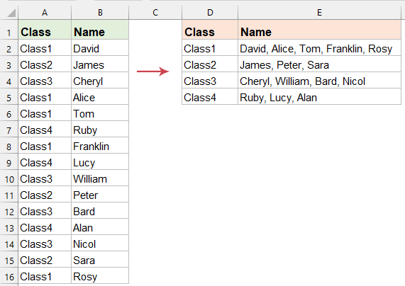
Voer in de doelcel de volgende formule in en sleep de formule naar beneden als je deze ook op andere rijen wilt toepassen. Alle overeenkomende waarden worden geëxtraheerd en samengevoegd in één cel. Zie screenshot:
=TEXTJOIN(", ", TRUE, FILTER($B$2:$B$16, $A$2:$A$16=D2, ""))
- FILTER($B$2:$B$16, $A$2:$A$16=D2, ""): Dit deel van de formule controleert elke waarde in $A$2:$A$16; als deze overeenkomt met de waarde in D2, wordt de bijbehorende waarde in $B$2:$B$16 opgenomen in de resultaatarray.
- $B$2:$B$16: Het bereik waaruit de overeenkomende waarden worden opgehaald.
- $A$2:$A$16=D2: De voorwaarde waarop waarden worden geselecteerd - alleen die rijen waarin $A$2:$A$16 gelijk is aan de inhoud in D2 worden verwerkt.
- TEXTJOIN(", ", TRUE, ...): Deze functie neemt de uitkomst van de FILTER-functie (een array van matches) en voegt ze samen tot één tekststring, gescheiden door het opgegeven scheidingsteken (komma en spatie), terwijl automatisch lege invoer worden genegeerd.
- ", ": Stelt komma en spatie in als scheidingsteken; je kunt dit symbool naar wens wijzigen, bijvoorbeeld puntkomma's of regeleinden gebruiken.
- TRUE: Zorgt ervoor dat lege cellen worden genegeerd in het samenvoegingsproces, zodat je een netjes opgemaakte uitkomst krijgt.
Speciale opmerking: Deze methode vereist Excel 365 of 2021 en werkt niet in oudere versies (bijv. Excel 2019, 2016 of eerder). Controleer altijd je Excel-versie voordat je deze methode toepast.
Tip: Als je zoekwaarde (bijv. D2) verandert of er worden extra overeenkomende items toegevoegd aan het gegevensbereik, dan wordt het resultaat automatisch bijgewerkt zonder extra stappen nodig.
Potentiële beperkingen: Bij zeer grote datasets kan de formuleberekeningstijd toenemen. Gebruikers moeten er ook voor zorgen dat er geen samengevoegde cellen zijn in het zoek- of resultaatbereik, omdat deze formulefouten kunnen veroorzaken.
Zoek en samenvoeg meerdere overeenkomstige waarden met Kutools voor Excel
Als je ingebouwde formulemethoden lastig vindt of je versie van Excel ondersteunt geen geavanceerde functies zoals TEXTJOIN en FILTER, biedt Kutools voor Excel een gebruiksvriendelijke grafische oplossing. De Eén-op-veel-zoeken-functie in Kutools maakt het mogelijk om met een paar stappen meerdere overeenkomstige resultaten te zoeken en samen te voegen, zodat het geschikt is voor zowel beginners als gevorderde gebruikers. Met Kutools hoef je geen ingewikkelde formules of codes te schrijven, en het is vooral handig bij het omgaan met grote of variabele datasets die herhaalde zoekacties en aggregaties vereisen.
Nadat je Kutools voor Excel hebt geïnstalleerd, volg je de onderstaande stappen:
Klik op Kutools > Super ZOEKEN > Eén-op-veel-zoeken (meerdere resultaten retourneren) om het instelvenster te openen. In dit venster kun je snel je zoek- en uitvoerinstellingen configureren met behulp van de volgende stappen:
- Selecteer je doeluitvoercellen voor de samengevoegde resultaten en de cellen die de waarden bevatten die je wilt zoeken;
- Geef het tabelbereik aan dat zowel de zoeksleutel als de resultaatkolommen bevat;
- Specificeer welke kolom de zoeksleutels bevat (Sleutelkolom) en de kolom waarvan de waarden zullen worden samengevoegd (Retourkolom);
- Klik op de OK-knop om je instellingen te bevestigen en de gegevens te verwerken.


Resultaat: Kutools zal nu alle overeenkomende en samengevoegde waarden in je geselecteerde uitvoercel weergeven. Zie screenshot:
Deze methode wordt ten zeerste aanbevolen voor wie liever vanuit de Excel-interface werkt zonder complexe formules of code. Het vermindert ook de kans op formulefouten en verbetert de productiviteit bij het afhandelen van repetitieve zoeken en samenvoegtaken.
Zoek en samenvoeg meerdere overeenkomstige waarden met een door de gebruiker gedefinieerde functie
Voor gebruikers die bedreven zijn in VBA (Visual Basic for Applications), of die oudere Excel-versies gebruiken die geen ondersteuning bieden voor dynamische matrices of de FILTER-functie, kun je een aangepaste door de gebruiker gedefinieerde functie (UDF) maken om flexibele samenvoeging van meerdere resultaten te bereiken. Deze methode is universeel compatibel met alle Excel-versies en kan worden aangepast aan specifieke scheidingstekensymbolen of voorwaarden.
1. Houd de toetsen ALT + F11 ingedrukt om het Microsoft Visual Basic for Applications venster te openen.
2. Klik op Invoegen > Module en plak de volgende code in het modulevenster.
VBA-code: Zoek en samenvoeg meerdere overeenkomende waarden in een cel
Function ConcatenateMatches(LookupValue As String, LookupRange As Range, ReturnRange As Range, Optional Delimiter As String = ", ") As String
'Updateby Extendoffice
    Dim Cell As Range
    Dim Result As String
    Result = ""
    For Each Cell In LookupRange
        If Cell.Value = LookupValue Then
            Result = Result & Cell.Offset(0, ReturnRange.Column - LookupRange.Column).Value & Delimiter
        End If
    Next Cell
    If Result <> "" Then
        Result = Left(Result, Len(Result) - Len(Delimiter))
    End If
    ConcatenateMatches = Result
End Function
3. Sla op en sluit de VBA-editor. Ga terug naar je werkblad en gebruik deze UDF door de formule in te voeren: =ConcatenateMatches(D2, $A$2:$A$16, $B$2:$B$16) in een lege cel waar je je resultaat wilt. Sleep de vulgreep naar beneden om de formule indien nodig naar andere cellen te kopiëren. Alle overeenkomende waarden op basis van een specifieke zoekwaarde worden geretourneerd en samengevoegd in één cel, gescheiden door een komma en spatie. Zie screenshot:

- D2: De zoekwaarde die in je dataset moet worden gematcht (LookupValue).
- A2:A16: Het bereik waarin de functie zoekt naar de zoekwaarde (LookupRange).
- B2:B16: Het bereik dat de waarden bevat om samen te voegen wanneer de zoekwaarde overeenkomt (ReturnRange).
Zoek en samenvoeg meerdere overeenkomstige waarden met VBA-code
Voor scenario's waarin herhaaldelijk gebruik wordt vereist of voor wie UDF's in werkbladcellen wil vermijden, kun je een kant-en-klare VBA-macro gebruiken om resultaten direct samen te voegen. Deze methode werkt goed in gedeelde omgevingen waar niet alle gebruikers dezelfde versie of invoegtoepassingen hebben.
1. Klik op Ontwikkelaarstools > Visual Basic om de VBA-editor te openen.
2. Klik in het VBA-venster op Invoegen > Module en plak deze code in de module:
Sub VLookupAndConcatenate()
    Dim ws As Worksheet
    Dim dataRange As Range, lookupRange As Range, resultRange As Range
    Dim dict As Object
    Dim i As Long, lastRow As Long
    Dim lookupValue As Variant, result As String
    Dim delimiter As String
    delimiter = ", "
    Set dict = CreateObject("Scripting.Dictionary")
    Set ws = ActiveSheet
    On Error Resume Next
    Set dataRange = Application.InputBox( _
        Prompt:="Please select the data range (contains lookup column and result column)", _
        Title:="Select Data Range", _
        Type:=8)
    On Error GoTo 0
    If dataRange Is Nothing Then Exit Sub
    On Error Resume Next
    Set lookupRange = Application.InputBox( _
        Prompt:="Please select the lookup range (single column)", _
        Title:="Select Lookup Range", _
        Type:=8)
    On Error GoTo 0
    If lookupRange Is Nothing Then Exit Sub
    On Error Resume Next
    Set resultRange = Application.InputBox( _
        Prompt:="Please select the starting cell for results output", _
        Title:="Select Output Location", _
        Type:=8)
    On Error GoTo 0
    If resultRange Is Nothing Then Exit Sub
    resultRange.Resize(lookupRange.Rows.Count, 1).ClearContents
    For i = 1 To dataRange.Rows.Count
        lookupValue = dataRange.Cells(i, 1).Value
        If Not dict.Exists(lookupValue) Then
            dict.Add lookupValue, dataRange.Cells(i, 2).Value
        Else
            dict(lookupValue) = dict(lookupValue) & delimiter & dataRange.Cells(i, 2).Value
        End If
    Next i
    For i = 1 To lookupRange.Rows.Count
        lookupValue = lookupRange.Cells(i, 1).Value
        If dict.Exists(lookupValue) Then
            resultRange.Cells(i, 1).Value = dict(lookupValue)
        Else
            resultRange.Cells(i, 1).Value = "Not Found"
        End If
    Next i
    MsgBox "Operation completed! Processed " & lookupRange.Rows.Count & " lookup values.", vbInformation
End Sub
3. Klik op de ![]() knop om de macro uit te voeren. De invoervelden vragen je om je gegevensbereik, zoekbereik en resultaatbereik te selecteren. Het samengevoegde resultaat wordt vervolgens direct weergegeven in de geselecteerde uitvoercellen.
knop om de macro uit te voeren. De invoervelden vragen je om je gegevensbereik, zoekbereik en resultaatbereik te selecteren. Het samengevoegde resultaat wordt vervolgens direct weergegeven in de geselecteerde uitvoercellen.
Deze macrobenadering is vooral handig als je vaak meerdere samenvoegzoekacties uitvoert met verschillende waarden, omdat het voorkomt dat je werkblad volloopt met UDF-aanroepen.
Je kunt gemakkelijk het scheidingsteken in de code aanpassen indien nodig, en de macro uitbreiden om resultaten uit te voeren naar een cel of bestand volgens je workflow.
Het samenvoegen van meerdere overeenkomstige waarden in Excel is mogelijk met verschillende benaderingen, elk met specifieke voordelen afhankelijk van je situatie. Of je nu kiest voor dynamische matrixformules, invoegtoepassingen zoals Kutools voor Excel of VBA-gebaseerde methoden, je verbetert je vermogen om gegroepeerde gegevens efficiënt te analyseren en weer te geven. Afhankelijk van de grootte en complexiteit van je dataset, overweeg dan welke benadering de optimale prestaties en onderhoudbaarheid biedt voor jou of je team. In dagelijkse operaties, controleer op gegevensconsistentie, vermijd samengevoegde cellen en verifieer referentiebereiken voor de beste resultaten. Als je fouten tegenkomt in formuleberekeningen, controleer dan of je bereiken overeenkomen met de gegevens en of je de juiste formule-invoermethode gebruikt voor je Excel-versie.
Voor meer geavanceerde Excel-technieken en een breed scala aan praktische handleidingen, bezoek onze uitgebreide tutorialbibliotheek.
Beste productiviteitstools voor Office
Verbeter je Excel-vaardigheden met Kutools voor Excel en ervaar ongeëvenaarde efficiëntie. Kutools voor Excel biedt meer dan300 geavanceerde functies om je productiviteit te verhogen en tijd te besparen. Klik hier om de functie te kiezen die je het meest nodig hebt...
Office Tab brengt een tabbladinterface naar Office en maakt je werk veel eenvoudiger
- Activeer tabbladbewerking en -lezen in Word, Excel, PowerPoint, Publisher, Access, Visio en Project.
- Open en maak meerdere documenten in nieuwe tabbladen van hetzelfde venster, in plaats van in nieuwe vensters.
- Verhoog je productiviteit met50% en bespaar dagelijks honderden muisklikken!
Alle Kutools-invoegtoepassingen. Eén installatieprogramma
Kutools for Office-suite bundelt invoegtoepassingen voor Excel, Word, Outlook & PowerPoint plus Office Tab Pro, ideaal voor teams die werken met Office-toepassingen.
- Alles-in-één suite — invoegtoepassingen voor Excel, Word, Outlook & PowerPoint + Office Tab Pro
- Eén installatieprogramma, één licentie — in enkele minuten geïnstalleerd (MSI-ready)
- Werkt beter samen — gestroomlijnde productiviteit over meerdere Office-toepassingen
- 30 dagen volledige proef — geen registratie, geen creditcard nodig
- Beste prijs — bespaar ten opzichte van losse aanschaf van invoegtoepassingen