Hoe cellen samen te voegen als er dezelfde waarde bestaat in een andere kolom in Excel?
Zoals te zien is in de onderstaande schermafbeelding, als u cellen in de tweede kolom wilt samenvoegen op basis van dezelfde waarden in de eerste kolom, zijn er verschillende methoden die u kunt gebruiken. In dit artikel introduceren we drie manieren om deze taak uit te voeren.

Cellen samenvoegen met formules en filter als er dezelfde waarde is
De volgende formules helpen bij het samenvoegen van de overeenkomstige cellen in één kolom op basis van overeenkomende waarden in een andere kolom.
1. Selecteer een lege cel naast de tweede kolom (hier selecteren we cel C2), voer de formule =ALS(A2<>A1;B2;C1 & "," & B2) in de formulebalk in, en druk vervolgens op de Enter-toets.

2. Selecteer vervolgens cel C2 en sleep de vulgreep naar beneden naar de cellen die u wilt samenvoegen.

3. Voer de formule =ALS(A2<>A3;SAMENVOEGEN(A2;",""";C2;""");"") in cel D2 in en sleep de vulgreep naar de resterende cellen.

4. Selecteer cel D1 en klik op Gegevens > Filter. Zie screenshot:

5. Klik op de vervolgkeuzepijl in cel D1, vink het vakje (Leeg) uit en klik vervolgens op de knop OK.

U ziet dat de cellen worden samengevoegd als de waarden in de eerste kolom hetzelfde zijn.

Opmerking: Om de bovenstaande formules succesvol te gebruiken, moeten dezelfde waarden in kolom A continu zijn.
Cellen eenvoudig samenvoegen met Kutools voor Excel (enkele klikken)
De hierboven beschreven methode vereist het maken van twee hulpkolommen en omvat meerdere stappen, wat mogelijk onhandig kan zijn. Als u op zoek bent naar een eenvoudigere manier, overweeg dan het gebruik van het Geavanceerd samenvoegen van rijen-hulpprogramma van Kutools voor Excel. Met slechts een paar klikken kunt u cellen samenvoegen met een specifiek scheidingsteken, waardoor het proces snel en probleemloos verloopt.
1. Klik op Kutools > Samenvoegen & Splitsen > Geavanceerd samenvoegen van rijen om deze functie in te schakelen.
2. In het dialoogvenster Geavanceerd samenvoegen van rijen hoeft u alleen maar:
- Selecteer het bereik dat u wilt samenvoegen;
- Stel de kolom met dezelfde waarden in als de Sleutelkolom.
- Specificeer een scheidingsteken om de cellen samen te voegen.
- Klik op OK.
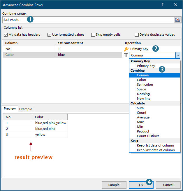
Resultaat

Kutools voor Excel - Boost Excel met meer dan 300 essentiële tools. Geniet van permanent gratis AI-functies! Nu verkrijgen
- Voor meer informatie over deze functie, bekijk dit artikel: Snel dezelfde waarden of dubbele rijen combineren in Excel
Cellen samenvoegen met VBA-code als er dezelfde waarde is
U kunt ook VBA-code gebruiken om cellen in een kolom samen te voegen als er dezelfde waarde bestaat in een andere kolom.
1. Druk op Alt + F11 om het venster Microsoft Visual Basic Applications te openen.
2. Klik in het venster Microsoft Visual Basic Applications op Invoegen > Module. Kopieer en plak vervolgens onderstaande code in het Module-venster.
VBA-code: cellen samenvoegen als er dezelfde waarden zijn
Sub ConcatenateCellsIfSameValues()
	Dim xCol As New Collection
	Dim xSrc As Variant
	Dim xRes() As Variant
	Dim I As Long
	Dim J As Long
	Dim xRg As Range
	xSrc    = Range("A1", Cells(Rows.Count, "A").End(xlUp)).Resize(, 2)
	Set xRg = Range("D1")
	On Error Resume Next
	For I = 2 To UBound(xSrc)
		xCol.Add xSrc(I, 1), TypeName(xSrc(I, 1)) & CStr(xSrc(I, 1))
	Next I
	On Error GoTo 0
	ReDim xRes(1 To xCol.Count + 1, 1 To 2)
	xRes(1, 1) = "No"
	xRes(1, 2) = "Combined Color"
	For I = 1 To xCol.Count
		xRes(I + 1, 1) = xCol(I)
		For J = 2 To UBound(xSrc)
			If xSrc(J, 1) = xRes(I + 1, 1) Then
				xRes(I + 1, 2) = xRes(I + 1, 2) & ", " & xSrc(J, 2)
			End If
		Next J
		xRes(I + 1, 2) = Mid(xRes(I + 1, 2), 2)
	Next I
	Set xRg = xRg.Resize(UBound(xRes, 1), UBound(xRes, 2))
	xRg.NumberFormat = "@"
	xRg = xRes
	xRg.EntireColumn.AutoFit
End SubOpmerkingen:
3. Druk op de F5-toets om de code uit te voeren, daarna krijgt u de samengevoegde resultaten in het opgegeven bereik.

Demo: Cellen eenvoudig samenvoegen met Kutools voor Excel
Beste productiviteitstools voor Office
Verbeter je Excel-vaardigheden met Kutools voor Excel en ervaar ongeëvenaarde efficiëntie. Kutools voor Excel biedt meer dan300 geavanceerde functies om je productiviteit te verhogen en tijd te besparen. Klik hier om de functie te kiezen die je het meest nodig hebt...
Office Tab brengt een tabbladinterface naar Office en maakt je werk veel eenvoudiger
- Activeer tabbladbewerking en -lezen in Word, Excel, PowerPoint, Publisher, Access, Visio en Project.
- Open en maak meerdere documenten in nieuwe tabbladen van hetzelfde venster, in plaats van in nieuwe vensters.
- Verhoog je productiviteit met50% en bespaar dagelijks honderden muisklikken!
Alle Kutools-invoegtoepassingen. Eén installatieprogramma
Kutools for Office-suite bundelt invoegtoepassingen voor Excel, Word, Outlook & PowerPoint plus Office Tab Pro, ideaal voor teams die werken met Office-toepassingen.
- Alles-in-één suite — invoegtoepassingen voor Excel, Word, Outlook & PowerPoint + Office Tab Pro
- Eén installatieprogramma, één licentie — in enkele minuten geïnstalleerd (MSI-ready)
- Werkt beter samen — gestroomlijnde productiviteit over meerdere Office-toepassingen
- 30 dagen volledige proef — geen registratie, geen creditcard nodig
- Beste prijs — bespaar ten opzichte van losse aanschaf van invoegtoepassingen