Hoe vlookup om meerdere waarden in één cel in Excel te retourneren?
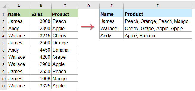
Normaal gesproken kunt u in Excel, wanneer u de functie VERT.ZOEKEN gebruikt, als er meerdere waarden zijn die aan de criteria voldoen, gewoon de eerste krijgen. Maar soms wilt u alle corresponderende waarden die aan de criteria voldoen, in één cel retourneren zoals in het onderstaande screenshot, hoe zou u dit kunnen oplossen?
- Vlookup om alle overeenkomende waarden in één cel te retourneren
- Vlookup om alle overeenkomende waarden zonder duplicaten in één cel te retourneren
Vlookup om meerdere waarden in één cel te retourneren met door de gebruiker gedefinieerde functie
- Vlookup om alle overeenkomende waarden in één cel te retourneren
- Vlookup om alle overeenkomende waarden zonder duplicaten in één cel te retourneren
Vlookup om meerdere waarden in één cel te retourneren met een handige functie
Vlookup om meerdere waarden in één cel te retourneren met de TEXTJOIN-functie (Excel 2019 en Office 365)
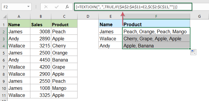
Als je de hogere versie van Excel hebt, zoals Excel 2019 en Office 365, is er een nieuwe functie - TEKSTJOINMet deze krachtige functie kunt u snel alle overeenkomende waarden opvouwen en in één cel retourneren.
Vlookup om alle overeenkomende waarden in één cel te retourneren
Pas de onderstaande formule toe in een lege cel waar u het resultaat wilt plaatsen en druk vervolgens op Ctrl + Shift + Enter toetsen samen om het eerste resultaat te krijgen en sleep vervolgens de vulgreep naar de cel waarin u deze formule wilt gebruiken, en u krijgt alle bijbehorende waarden zoals hieronder afgebeeld:
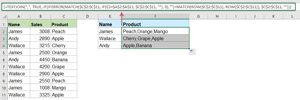
Vlookup om alle overeenkomende waarden zonder duplicaten in één cel te retourneren
Als u alle overeenkomende waarden wilt retourneren op basis van de opzoekgegevens zonder duplicaten, kan de onderstaande formule u helpen.
Kopieer en plak de volgende formule in een lege cel en druk op Ctrl + Shift + Enter sleutels samen om het eerste resultaat te krijgen, en kopieer vervolgens deze formule om andere cellen te vullen, en je krijgt alle corresponderende waarden zonder de dulpicatie zoals onderstaand screenshot getoond:
Vlookup om meerdere waarden in één cel te retourneren met door de gebruiker gedefinieerde functie
De bovenstaande TEXTJOIN-functie is alleen beschikbaar voor Excel 2019 en Office 365, als u andere lagere Excel-versies heeft, moet u enkele codes gebruiken om deze taak te voltooien.
Vlookup om alle overeenkomende waarden in één cel te retourneren
1. Houd de ALT + F11 toetsen, en het opent de Microsoft Visual Basic voor toepassingen venster.
2. Klikken Invoegen > Moduleen plak de volgende code in het Module Venster.
VBA-code: Vlookup om meerdere waarden in één cel te retourneren
Function ConcatenateIf(CriteriaRange As Range, Condition As Variant, ConcatenateRange As Range, Optional Separator As String = ",") As Variant
'Updateby Extendoffice
Dim xResult As String
On Error Resume Next
If CriteriaRange.Count <> ConcatenateRange.Count Then
    ConcatenateIf = CVErr(xlErrRef)
    Exit Function
End If
For i = 1 To CriteriaRange.Count
    If CriteriaRange.Cells(i).Value = Condition Then
        xResult = xResult & Separator & ConcatenateRange.Cells(i).Value
    End If
Next i
If xResult <> "" Then
    xResult = VBA.Mid(xResult, VBA.Len(Separator) + 1)
End If
ConcatenateIf = xResult
Exit Function
End Function
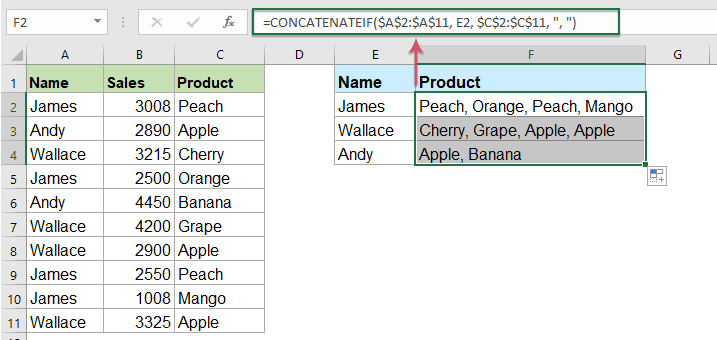
3. Sla vervolgens deze code op en sluit deze, ga terug naar het werkblad en voer deze formule in: =CONCATENATEIF($A$2:$A$11, E2, $C$2:$C$11, ", ") in een specifieke lege cel waar u het resultaat wilt plaatsen en sleep vervolgens de vulgreep naar beneden om alle overeenkomstige waarden in één cel te krijgen die u wilt, zie screenshot:
Vlookup om alle overeenkomende waarden zonder duplicaten in één cel te retourneren
Gebruik de onderstaande code om de duplicaten in de geretourneerde overeenkomende waarden te negeren.
1. Houd de Alt + F11 toetsen om de te openen Microsoft Visual Basic voor toepassingen venster.
2. Klikken Invoegen > Moduleen plak de volgende code in het Module Venster.
VBA-code: Vlookup en retourneer meerdere unieke overeenkomende waarden in één cel
Function MultipleLookupNoRept(Lookupvalue As String, LookupRange As Range, ColumnNumber As Integer)
'Updateby Extendoffice
    Dim xDic As New Dictionary
    Dim xRows As Long
    Dim xStr As String
    Dim i As Long
    On Error Resume Next
    xRows = LookupRange.Rows.Count
    For i = 1 To xRows
        If LookupRange.Columns(1).Cells(i).Value = Lookupvalue Then
            xDic.Add LookupRange.Columns(ColumnNumber).Cells(i).Value, ""
        End If
    Next
    xStr = ""
    MultipleLookupNoRept = xStr
    If xDic.Count > 0 Then
        For i = 0 To xDic.Count - 1
            xStr = xStr & xDic.Keys(i) & ","
        Next
        MultipleLookupNoRept = Left(xStr, Len(xStr) - 1)
    End If
End Function
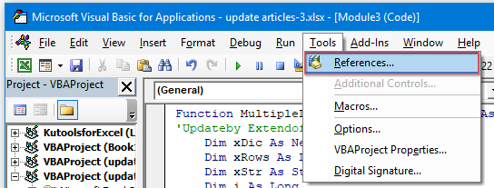
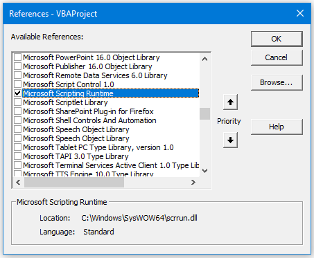
3. Nadat u de code heeft ingevoerd, klikt u op Tools > Referenties in de geopende Microsoft Visual Basic voor toepassingen venster, en dan, in de pop-out Referenties - VBAProject dialoogvenster, vink aan Microsoft Scripting-runtime optie in het Beschikbare referenties keuzelijst, zie screenshots:
 |
 |
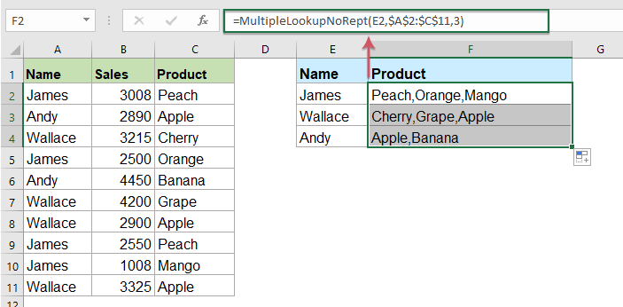
4. Dan klikken OK om het dialoogvenster te sluiten, slaat u het codevenster op en sluit u het, keert u terug naar het werkblad en voert u deze formule in: =MultipleLookupNoRept(E2,$A$2:$C$11,3) into a blank cell where you want to output the result, and then drag the fill hanlde down to get all matching values, see screenshot:
Vlookup om meerdere waarden in één cel te retourneren met een handige functie
Als u ons Kutools for Excel, Met Geavanceerd Combineer rijen functie, kunt u snel de rijen samenvoegen of combineren op basis van dezelfde waarde en enkele berekeningen uitvoeren als u nodig hebt.
Na het installeren van Kutools for Excelgaat u als volgt te werk:
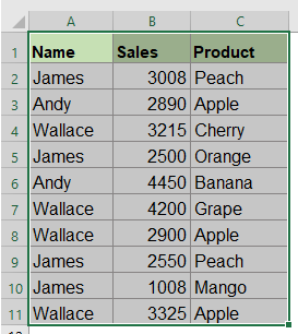
1. Selecteer het gegevensbereik waarvoor u de ene kolomgegevens wilt combineren op basis van een andere kolom.
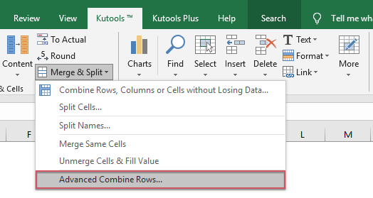
2. Klikken Kutools > Samenvoegen en splitsen > Geavanceerd Combineer rijen, zie screenshot:
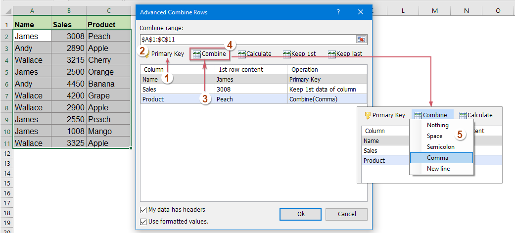
3. In de pop-out Geavanceerd Combineer rijen dialoog venster:
- Klik op de naam van de sleutelkolom die u wilt combineren op basis van, en klik vervolgens op Hoofdsleutel
- Klik vervolgens op een andere kolom waarvan u de gegevens wilt combineren op basis van de sleutelkolom, en klik op Combineren om een scheidingsteken te kiezen voor het scheiden van de gecombineerde gegevens.
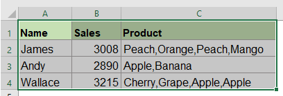
4. Dan klikken OK knop, en je krijgt de volgende resultaten:
 |
 |
Download en gratis proef Kutools voor Excel nu!
Meer relatieve artikelen:
- VERT.ZOEKEN-functie met enkele eenvoudige en geavanceerde voorbeelden
- In Excel is de functie VERT.ZOEKEN een krachtige functie voor de meeste Excel-gebruikers, die wordt gebruikt om naar een waarde uiterst links in het gegevensbereik te zoeken en een overeenkomende waarde in dezelfde rij te retourneren vanuit een kolom die u hebt opgegeven. Deze tutorial heeft het over het gebruik van de functie VERT.ZOEKEN met enkele basis- en geavanceerde voorbeelden in Excel.
- Retourneer meerdere overeenkomende waarden op basis van een of meerdere criteria
- Normaal gesproken is het opzoeken van een specifieke waarde en het retourneren van het overeenkomende item voor de meesten van ons eenvoudig met de functie VERT.ZOEKEN. Maar heb je ooit geprobeerd om meerdere overeenkomende waarden te retourneren op basis van een of meer criteria? In dit artikel zal ik enkele formules introduceren om deze complexe taak in Excel op te lossen.
- Bekijk en retourneer meerdere waarden verticaal
- Normaal gesproken kunt u de functie Vlookup gebruiken om de eerste overeenkomstige waarde te krijgen, maar soms wilt u alle overeenkomende records retourneren op basis van een specifiek criterium. In dit artikel zal ik het hebben over het opvullen en retourneren van alle overeenkomende waarden verticaal, horizontaal of in één enkele cel.
- Bekijk en retourneer meerdere waarden uit de vervolgkeuzelijst
- Hoe kunt u in Excel meerdere overeenkomstige waarden opvragen en retourneren uit een vervolgkeuzelijst, wat betekent dat wanneer u één item uit de vervolgkeuzelijst kiest, alle relatieve waarden tegelijk worden weergegeven. In dit artikel zal ik de oplossing stap voor stap introduceren.
Beste Office-productiviteitstools
Geef uw Excel-vaardigheden een boost met Kutools voor Excel en ervaar efficiëntie als nooit tevoren. Kutools voor Excel biedt meer dan 300 geavanceerde functies om de productiviteit te verhogen en tijd te besparen. Klik hier om de functie te krijgen die u het meest nodig heeft...
")
Office-tabblad Brengt een interface met tabbladen naar Office en maakt uw werk veel gemakkelijker
- Schakel bewerken en lezen met tabbladen in Word, Excel, PowerPoint in, Publisher, Access, Visio en Project.
- Open en maak meerdere documenten in nieuwe tabbladen van hetzelfde venster in plaats van in nieuwe vensters.
- Verhoogt uw productiviteit met 50% en vermindert honderden muisklikken voor u elke dag!
")