Hoe vind je de eerste of laatste vrijdag van elke maand in Excel?
Normaal gesproken is vrijdag de laatste werkdag van de maand. Hoe kun je de eerste of laatste vrijdag vinden op basis van een gegeven datum in Excel? In dit artikel leiden we je door het gebruik van twee formules om de eerste of laatste vrijdag van elke maand te vinden.
Zoek de eerste vrijdag van een maand
Zoek de laatste vrijdag van een maand
Zoek de eerste vrijdag van een maand
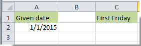
Bijvoorbeeld, er is een gegeven datum 1/1/2015 die zich in cel A2 bevindt, zoals in de onderstaande schermafbeelding te zien is. Als je de eerste vrijdag van de maand wilt vinden op basis van de gegeven datum, doe dan het volgende.
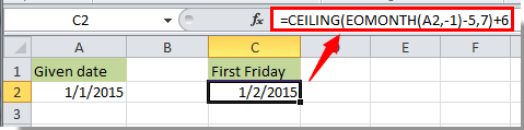
1. Selecteer een cel om het resultaat weer te geven. Hier selecteren we cel C2.
2. Kopieer en plak de onderstaande formule erin en druk vervolgens op de Enter-toets.
=CEILING(EOMONTH(A2,-1)-5,7)+6
Opmerkingen:
Zoek de laatste vrijdag van een maand
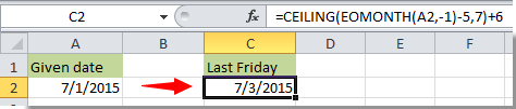
De gegeven datum 1/1/2015 bevindt zich in cel A2. Om de laatste vrijdag van deze maand in Excel te vinden, doe dan het volgende.
1. Selecteer een cel, kopieer de onderstaande formule erin en druk vervolgens op de Enter-toets om het resultaat te krijgen.
=DATE(YEAR(A2),MONTH(A2)+1,0)+MOD(-WEEKDAY(DATE(YEAR(A2),MONTH(A2)+1,0),2)-2,-7)

Opmerking: Je kunt A2 in de formule wijzigen naar de referentiecel van je gegeven datum.
Gerelateerde artikelen:
- Hoe vind je de laagste en hoogste 5 waarden in een lijst in Excel?
- Hoe vind je of controleer je of een specifiek werkboek geopend is of niet in Excel?
- Hoe kom je erachter of een cel in een andere cel wordt gerefereerd in Excel?
- Hoe vind je de dichtstbijzijnde datum bij vandaag in een lijst in Excel?
Beste productiviteitstools voor Office
Verbeter je Excel-vaardigheden met Kutools voor Excel en ervaar ongeëvenaarde efficiëntie. Kutools voor Excel biedt meer dan300 geavanceerde functies om je productiviteit te verhogen en tijd te besparen. Klik hier om de functie te kiezen die je het meest nodig hebt...
Office Tab brengt een tabbladinterface naar Office en maakt je werk veel eenvoudiger
- Activeer tabbladbewerking en -lezen in Word, Excel, PowerPoint, Publisher, Access, Visio en Project.
- Open en maak meerdere documenten in nieuwe tabbladen van hetzelfde venster, in plaats van in nieuwe vensters.
- Verhoog je productiviteit met50% en bespaar dagelijks honderden muisklikken!
Alle Kutools-invoegtoepassingen. Eén installatieprogramma
Kutools for Office-suite bundelt invoegtoepassingen voor Excel, Word, Outlook & PowerPoint plus Office Tab Pro, ideaal voor teams die werken met Office-toepassingen.
- Alles-in-één suite — invoegtoepassingen voor Excel, Word, Outlook & PowerPoint + Office Tab Pro
- Eén installatieprogramma, één licentie — in enkele minuten geïnstalleerd (MSI-ready)
- Werkt beter samen — gestroomlijnde productiviteit over meerdere Office-toepassingen
- 30 dagen volledige proef — geen registratie, geen creditcard nodig
- Beste prijs — bespaar ten opzichte van losse aanschaf van invoegtoepassingen