Hoe voorwaardelijke opmaak toepassen op datums kleiner dan of groter dan vandaag in Excel?
Het beheren en volgen van tijdgevoelige informatie is cruciaal in veel Excel-taken, van projectplanning tot vervaldatums van facturen of het monitoren van deadlines. Een veelvoorkomende eis is om visueel onderscheid te maken tussen datums die eerder zijn dan vandaag of later dan vandaag. De voorwaardelijke opmaak in Excel stelt u in staat om dergelijke datums automatisch te markeren, zodat u snel verlopen taken of aankomende gebeurtenissen kunt herkennen zonder handmatig door de gegevens te scrollen. In deze handleiding leiden we u door verschillende praktische benaderingen om datums voor of na vandaag te markeren, inclusief ingebouwde Excel-tools en verbeterde oplossingen met Kutools voor Excel. U leert hoe u vervaldatums effectief kunt benadrukken, toekomstige activiteiten kunt markeren en overzicht kunt houden in uw spreadsheets, ongeacht uw gegevensvolume of update-behoeften.
- Markeer datums voor vandaag of in de toekomst met Voorwaardelijke Opmaak
- Markeer datums voor vandaag of in de toekomst met Kutools AI
- Markeer en analyseer datums met formules in een hulpkolom in Excel
Markeer datums voor vandaag of in de toekomst met Voorwaardelijke Opmaak
Stel dat u een kolom hebt met verschillende datums, zoals geïllustreerd in de onderstaande schermafbeelding. Als u datums wilt markeren die al verlopen zijn (vóór vandaag) of toekomstige datums wilt markeren om bij te houden en plannen te maken, kunt u gebruik maken van de voorwaardelijke opmaak in Excel met formules gebaseerd op de VANDAAG-functie. Deze functie is vooral waardevol bij het werken met dynamische gegevens, omdat de opmaak elke dag automatisch wordt bijgewerkt.

Selecteer eerst uw lijst met datums — in dit voorbeeld selecteert u cellen A2:A15. Klik op het tabblad Start op Voorwaardelijke Opmaak > Regels Beheren. Raadpleeg de onderstaande schermafbeelding voor richtlijnen:

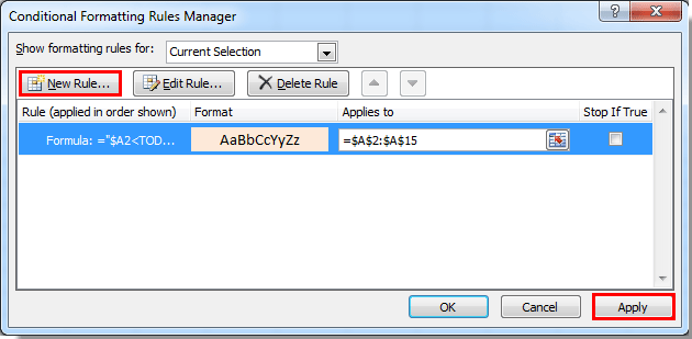
Zodra het dialoogvenster Voorwaardelijke Opmaakregels Manager verschijnt, klikt u op de knop Nieuwe Regel om een aangepaste regel te maken op basis van een formule.

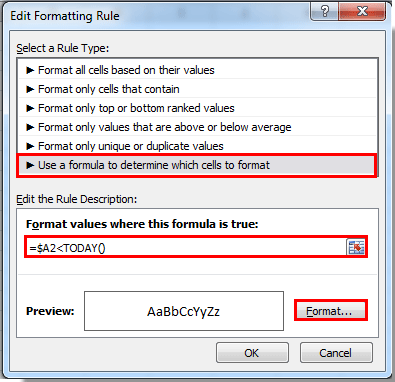
In het dialoogvenster Nieuwe Opmaakregel:
• Kies Gebruik een formule om te bepalen welke cellen te formatteren. Deze optie biedt flexibiliteit voor datumgerichte markering.
• Om datums ouder dan vandaag te markeren, kopieert en plakt u de volgende formule in het veld Formateer waarden waar deze formule waar is:
=$A2<TODAY()• Om datums na vandaag (bijvoorbeeld komende toekomstige datums) te markeren, gebruikt u deze formule:
=$A2>TODAY()• Klik vervolgens op de knop Opmaak om uw gewenste uiterlijk te definiëren (zoals de vulkleur of lettertypestijl wijzigen). Zie het voorbeeld:
Specificeer uw gewenste opmaak in het dialoogvenster Celopmaak instellen (bijvoorbeeld kies een kleur om vervaldatums of toekomstige datums te laten opvallen), en klik vervolgens op OK.
Terug in de Voorwaardelijke Opmaakregels Manager ziet u uw nieuwe regel vermeld. Om de regel te activeren, klikt u op Toepassen. Als u zowel vervallen als toekomstige datums wilt markeren, herhaalt u de stappen om een tweede regel toe te voegen met de andere formule. Wanneer u terugkeert naar de Regelsmanager, zullen nu beide regels zichtbaar zijn.
Na bevestiging met OK zal uw Excel-werkblad nu visueel onderscheid maken tussen datums voor en na vandaag, met duidelijke indicatoren om actie of aandacht te stimuleren. Zowel verlopen als toekomstige datums worden automatisch bijgewerkt wanneer dagen veranderen, zodat u altijd de meest relevante items in één oogopslag ziet.

Hier is het resultaat: datums eerder of later dan vandaag zijn nu gemarkeerd volgens uw formaatselectie, wat de controle en follow-up vereenvoudigt.

Tips en Waarschuwingen: Zorg ervoor dat uw datumcellen zijn opgemaakt als datums (niet als tekst) om ervoor te zorgen dat formules correct werken. Als u onverwachte resultaten ervaart, controleer dan uw datumformaat nogmaals. Voor zeer grote datasets kan voorwaardelijke opmaak de prestaties beïnvloeden, dus overweeg om de opmaakbereik indien mogelijk te beperken.
Markeer datums voor vandaag of in de toekomst met Kutools AI
Voor gebruikers die op zoek zijn naar een eenvoudigere, slimmere manier om verlopen of toekomstige datums te markeren, stroomlijnt Kutools AI voor Excel het proces. In plaats van handmatig voorwaardelijke opmaakregels te bouwen, kunt u Kutools AI direct instructies geven in gewone taal. Deze methode is ideaal als u regelmatig datums moet markeren, maar tijd wilt besparen of het instellen van formules wilt vermijden, of als u werkt in omgevingen waar nauwkeurigheid en efficiëntie van groot belang zijn.
Om Kutools AI te gebruiken voor het markeren van datums op basis van hun relatie met vandaag:
- Klik op 'Kutools' > 'AI Assistent' om het paneel 'Kutools AI Assistent' te openen, en voer vervolgens de volgende handelingen uit:
- Selecteer het datumgebied dat u wilt onderzoeken.
- Typ in het AI Assistent-paneel een opdracht zoals:
— Voor verlopen datums: Markeer de datums voor vandaag met lichtblauwe kleur in het geselecteerde bereik
— Voor toekomstige datums: Markeer de datums na vandaag met lichtblauwe kleur in het geselecteerde bereik - Druk op Enter of klik op Verzenden. Kutools AI zal uw verzoek analyseren. Zodra de verwerking is voltooid, klikt u op Uitvoeren om de opmaak automatisch toe te passen.
Kutools AI interpreteert automatisch uw bedoeling, kiest de juiste formules en formaten, bespaart u tijd en minimaliseert fouten bij handmatige configuratie. Deze aanpak is vooral nuttig in dynamische werkboeken, voor gebruikers die minder bekend zijn met formules, of voor hen die grote, vaak bijgewerkte datumbereiken beheren.
Waarschuwing: Kutools AI vereist internetverbinding en een up-to-date installatie van Kutools voor Excel.
Markeer en analyseer datums met hulpkolomformules in Excel
In veel praktijkgevallen wilt u misschien meer dan alleen kleurcodering — bijvoorbeeld filteren, sorteren of tellen van records op basis van of datums voor of na vandaag zijn. Het gebruik van hulpkolommen met Excel-formules stelt u in staat om dergelijke gevallen duidelijk te markeren en andere functies van Excel (zoals filters of draaitabellen) te gebruiken voor gedetailleerde analyses.
Voordelen: Makkelijk in te stellen, ondersteunt sorteren/filteren, werkt in alle Excel-versies zonder speciale rechten. Nadelen: Vereist extra ruimte voor hulpkolommen; biedt geen directe kleuring tenzij gecombineerd met voorwaardelijke opmaak.
Hier is hoe u een hulpkolom kunt gebruiken voor snelle datumanalyse:
1. Voeg een nieuwe kolom in naast uw datumbereik (bijvoorbeeld kolom B naast uw datums in A2:A15).
2. Typ in cel B2 (ervan uitgaande dat A2 uw eerste datum is) deze formule om verlopen datums te markeren:
=A2<TODAY()Deze formule retourneert WAAR als de datum in A2 voor vandaag is en ONWAAR anders.
3. Als alternatief, om toekomstige datums te markeren, gebruikt u:
=A2>TODAY()4. Druk op Enter om de formule te bevestigen, en sleep de handgreep naar beneden om de kolom te vullen voor alle rijen met datums. De WAAR/ONWAAR-resultaten kunnen nu worden gebruikt om records te sorteren of filteren op basis van verlopen of komende status.
Als u liever duidelijke tekstlabels hebt, vervang dan WAAR/ONWAAR door meer beschrijvende labels. Bijvoorbeeld:
=IF(A2<TODAY(),"Overdue",IF(A2>TODAY(),"Upcoming","Today"))Kopieer deze formule naar beneden naar alle relevante rijen indien nodig. U kunt filteren, sorteren of de kolom gebruiken als criterium in andere Excel-functies, zoals Voorwaardelijke Opmaak of Draaitabellen. Deze aanpak is vooral handig voor rapportages, dashboards of het voorbereiden van afdrukbare documenten.
Opmerking: Als uw datumkolom niet kolom A is, werk de verwijzing naar de cel in de formule dienovereenkomstig bij. Zorg ervoor dat uw gegevenstype voor datumcellen is ingesteld op datum, niet op tekst, om inconsistente resultaten te voorkomen.
Gerelateerde artikelen:
- Hoe voorwaardelijke opmaak toepassen op cellen op basis van de eerste letter/teken in Excel?
- Hoe voorwaardelijke opmaak toepassen op cellen die #na bevatten in Excel?
- Hoe voorwaardelijke opmaak of markeer de eerste herhaling in Excel?
- Hoe negatieve percentages in rood voorwaardelijk opmaken in Excel?
Snelle tips voor probleemoplossing: Als het markeren of de formules niet werken zoals bedoeld, controleer dan altijd uw datumopmaak en formulebereiken. Gebruik de Voorbeeldfunctie in Voorwaardelijke Opmaak om te controleren welke records worden beïnvloed, en controleer dubbel op dubbele regels die elkaar kunnen overlappen of tegenspreken. Voor grotere tabellen kunnen hulpkolommen of VBA-macros onderhoud stroomlijnen en tijd besparen wanneer frequent updates nodig zijn. Verken meerdere methoden om de workflow te vinden die het beste past bij uw scenario's.
Beste productiviteitstools voor Office
Verbeter je Excel-vaardigheden met Kutools voor Excel en ervaar ongeëvenaarde efficiëntie. Kutools voor Excel biedt meer dan300 geavanceerde functies om je productiviteit te verhogen en tijd te besparen. Klik hier om de functie te kiezen die je het meest nodig hebt...
Office Tab brengt een tabbladinterface naar Office en maakt je werk veel eenvoudiger
- Activeer tabbladbewerking en -lezen in Word, Excel, PowerPoint, Publisher, Access, Visio en Project.
- Open en maak meerdere documenten in nieuwe tabbladen van hetzelfde venster, in plaats van in nieuwe vensters.
- Verhoog je productiviteit met50% en bespaar dagelijks honderden muisklikken!
Alle Kutools-invoegtoepassingen. Eén installatieprogramma
Kutools for Office-suite bundelt invoegtoepassingen voor Excel, Word, Outlook & PowerPoint plus Office Tab Pro, ideaal voor teams die werken met Office-toepassingen.
- Alles-in-één suite — invoegtoepassingen voor Excel, Word, Outlook & PowerPoint + Office Tab Pro
- Eén installatieprogramma, één licentie — in enkele minuten geïnstalleerd (MSI-ready)
- Werkt beter samen — gestroomlijnde productiviteit over meerdere Office-toepassingen
- 30 dagen volledige proef — geen registratie, geen creditcard nodig
- Beste prijs — bespaar ten opzichte van losse aanschaf van invoegtoepassingen