Hoe waarden tussen twee datums in Excel optellen?
Wanneer er twee lijsten in uw werkblad staan zoals in de rechter screenshot te zien is, waarbij de ene lijst de datums bevat en de andere de waarden, en u wilt alleen de waarden optellen binnen een bereik van twee datums, bijvoorbeeld de waarden optellen tussen 4 maart 2014 en 10 mei 2014, hoe kunt u deze dan snel berekenen? Hier introduceer ik een formule om ze in Excel op te tellen.
- Waarden tussen twee datums optellen met formule in Excel
- Waarden tussen twee datums optellen met filter in Excel
Waarden tussen twee datums optellen met formule in Excel
Gelukkig is er een formule die de waarden tussen een bereik van twee datums in Excel kan optellen.
Selecteer een lege cel en typ de onderstaande formule in, en druk op de Enter-knop. U krijgt nu het berekende resultaat te zien. Zie screenshot:
=SOMMEN.ALS(B2:B8,A2:A8,">="&E2,A2:A8,"<="&E3)
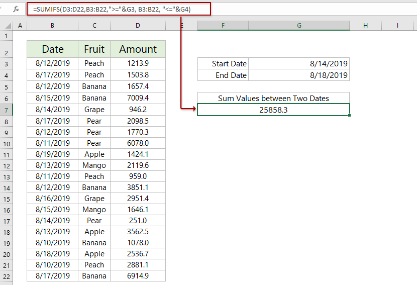
Opmerking: In bovenstaande formule,
- D3:D22 is de waarde-lijst die u wilt optellen
- B3:B22 is de datum-lijst waarop u gebaseerd wilt optellen
- G3 is de cel met de startdatum
- G4 is de cel met de einddatum
 | Formule te ingewikkeld om te onthouden? Sla de formule op als een AutoTekst-item om in de toekomst met slechts één klik te hergebruiken! Lees meer… Gratis proefversie |
Gemakkelijk gegevens optellen voor elk fiscaal jaar, elk halfjaar of elke week in Excel
De functie Speciale tijdsgroepering toevoegen aan draaitabel, aangeboden door Kutools voor Excel, voegt een hulpkolom toe om het fiscale jaar, halfjaar, weeknummer of dag van de week te berekenen op basis van de opgegeven datumkolom, en laat u gemakkelijk kolommen optellen, tellen of middelen op basis van de berekende resultaten in een nieuwe draaitabel.
Kutools voor Excel - Boost Excel met meer dan 300 essentiële tools. Geniet van permanent gratis AI-functies! Nu verkrijgen
Waarden tussen twee datums optellen met filter in Excel
Als u waarden tussen twee datums moet optellen en het datumbereik verandert vaak, kunt u een filter toevoegen voor een bepaald bereik en vervolgens de functie SUBTOTAAL gebruiken om binnen het gespecificeerde datumbereik in Excel op te tellen.
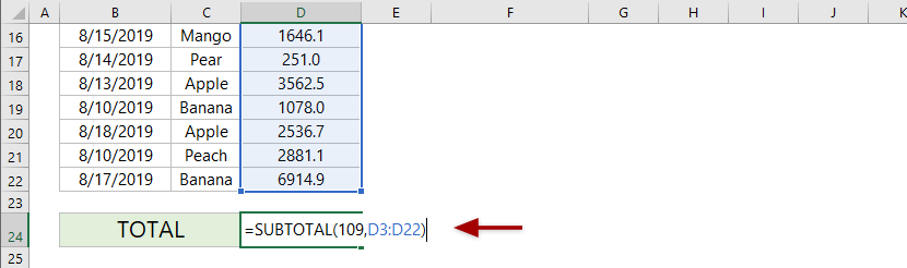
1. Selecteer een lege cel, voer onderstaande formule in en druk op de Enter-toets.
=SUBTOTAAL(109,D3:D22)
Opmerking: In bovenstaande formule betekent 109 som gefilterde waarden, D3:D22 geeft de waarde-lijst aan die u wilt optellen.
2. Selecteer de titel van het bereik en voeg een filter toe door te klikken op Gegevens > Filter.

3. Klik op het filterpictogram in de koptekst van de datumkolom en selecteer Datumfilters > Tussen. Typ in het dialoogvenster Aangepast Autofilter de startdatum en einddatum zoals u nodig hebt, en klik op de OK knop. De totale waarde zal automatisch veranderen op basis van de gefilterde waarden.
Gerelateerde artikelen:
Beste productiviteitstools voor Office
Verbeter je Excel-vaardigheden met Kutools voor Excel en ervaar ongeëvenaarde efficiëntie. Kutools voor Excel biedt meer dan300 geavanceerde functies om je productiviteit te verhogen en tijd te besparen. Klik hier om de functie te kiezen die je het meest nodig hebt...
Office Tab brengt een tabbladinterface naar Office en maakt je werk veel eenvoudiger
- Activeer tabbladbewerking en -lezen in Word, Excel, PowerPoint, Publisher, Access, Visio en Project.
- Open en maak meerdere documenten in nieuwe tabbladen van hetzelfde venster, in plaats van in nieuwe vensters.
- Verhoog je productiviteit met50% en bespaar dagelijks honderden muisklikken!
Alle Kutools-invoegtoepassingen. Eén installatieprogramma
Kutools for Office-suite bundelt invoegtoepassingen voor Excel, Word, Outlook & PowerPoint plus Office Tab Pro, ideaal voor teams die werken met Office-toepassingen.
- Alles-in-één suite — invoegtoepassingen voor Excel, Word, Outlook & PowerPoint + Office Tab Pro
- Eén installatieprogramma, één licentie — in enkele minuten geïnstalleerd (MSI-ready)
- Werkt beter samen — gestroomlijnde productiviteit over meerdere Office-toepassingen
- 30 dagen volledige proef — geen registratie, geen creditcard nodig
- Beste prijs — bespaar ten opzichte van losse aanschaf van invoegtoepassingen